Hi Community
I am working on a proof-of-concept workflow which merges Energy End Uses with a breakdown of Thermal Gains+Losses into a single pie-chart (Visualized using Conduit) and am looking for validation that this approach makes sense as a way to connect the breakdown of Thermal Gains+Losses with total cooling and heating energy.
The purpose of this workflow is to give designers a very early, high-level understanding of the major factors which contribute to building energy use and help to prioritize EEMs and future simulation studies. For example, if the result indicates that Solar Gain is high, the focus could be on shading. If conduction through walls and windows is high, increasing insulation studies and wall detailing could be an effective next step. The inspiration for this comes from the Energy Balance monthly chart component, but the intent here is to tie thermal gains+losses back to total energy use (impact on heating or cooling loads) and estimated EUI to put things in context.
My process was this:
Run an energy simulation in HB Open Studio using baseline/code level values to represent inputs known at a very early design stage. (The example shown is a 4650 m2 office building in Minneapolis, MN).
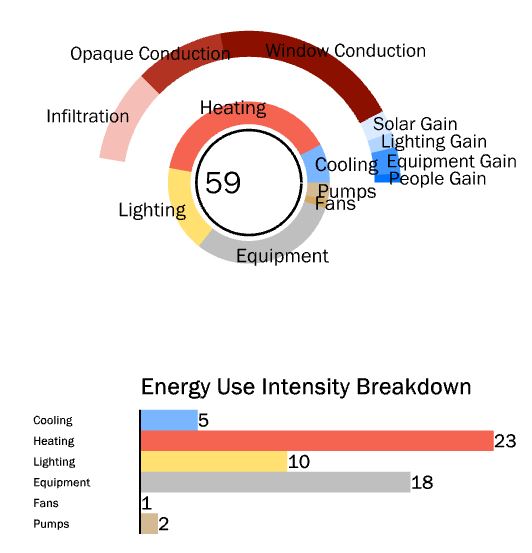
Generate EUI and Energy End Uses from Read EP Result (aggregated as annual kWh) to create the inner ring of the pie chart and EUI value:
Heating: 342,192 kWh (23 kBtu/sf/yr)
Cooling: 67,467 kWh (5 kBtu/sf/yr)
Electric Lighting: 150,481 kWh (10 kBtu/sf/yr)
Electric Equip: 264,808 kWh (18 kBtu/sf/yr)
Fans: 14338 kWh (1 kBtu/sf/yr)
Pumps: 30,555 kWh (2 kBtu/sf/yr)
Total EUI: 59
Pull in Thermal Gains+Losses values from Read EP Result and Read EP Surface results (annual).
*People Gain: 89,710 kWh *
*Equip Gain: 264,808 kWh *
*Lighting Gain: 150,481 kWh *
Solar Gain: 228,276 kWh
Glazing Conduction Loss: -201,930 kWh
Opaque Conduction Loss: -95,390 kWh
Infiltration Loss: -97,962 kWh
I then got the sum of both heat gains and heat losses, and divided each individual term (i.e. people gains, lighting gains, etc) by this sum of the category it is in (gain or loss) to generate % of total gain or loss each factor contributed to.
For example, for solar gain:
Annual Solar Heat gain (228,276 kWh)/(SUM of all gains (733,277 kWh) = 31% of total Cooling is attributed to Solar Gains.
*This is where I am looking for validation of approach
Lastly, I multiplied this ‘% of total heat gain or loss’ for each term by the EUI of either Heating (if it was a loss term) or Cooling (if it was a gain term) to be able to plot these ‘proportional EUI’ values on the pie chart to indicate Cooling and Heating breakdowns.
My questions:
Is my method, in Step 4 above, an effective way to quantify the thermal gains and losses relate to total cooling or heating load at a very early stage?
One more detailed question on Light and Equip terms: I am seeing in the .csv file from OS results that the values for Elec Lights and Elec Equip (total annual GJ) are the same as the Annual Sensible Heat Gains (GJ) for Lights and Equipment. Is this because almost all electric energy associated with these loads is emitted as heat? I’m confused about why electric energy for equip and lights vs heat emitted from equip and lights are not considered as separate terms when using the Monthly Energy Balance component, and why these values (elec load and heat gains) would be the same?
Please let me know if there is any thing I can clarify about this workflow, and thank you for your feedback!
Is my method, in Step 4 above, an effective way to quantify the thermal gains and losses relate to total cooling or heating load at a very early stage?
If I’m interpreting this correctly, the problem I see with this is that the sum of the annual component heating, and cooling loads (solar, equipment etc) is not equal to mechanical heating, cooling loads - since some of that energy is offset (or balanced) by passive cooling and heating, respectively, which cannot be correctly accounted for if you’re taking the annual sum.
In the monthly energy balance, if you subtract the total component sum by the passive offset it will approximate the mechanical energy. That’s why that representation is useful, it can break down the mechanical loads to it’s respective components. In this case, that won’t work because the aggregation over the year will not register specific passive offsets that occur at a sub-yearly intervals, that lead to the summed mechanical energy. Since you aren’t accounting for the correct passive offsets, the resulting annual breakdown is providing misleading information. So for example, let’s say you have +40 window conduction gain in summer, and -40 window conduction loss in the winter, and a -10 conduction loss from your walls. In sum this would result in 0 window conduction energy, and -10 wall conduction energy transfer. You would therefore conclude the wall R-value has a larger impact on the building energy, then the window U-value. It could work if at minimum you split your summed periods into two for the heating and cooling seasons.
One more detailed question on Light and Equip terms: I am seeing in the .csv file from OS results that the values for Elec Lights and Elec Equip (total annual GJ) are the same as the Annual Sensible Heat Gains (GJ) for Lights and Equipment. Is this because almost all electric energy associated with these loads is emitted as heat?
Yes, as per the 2nd law of thermodynamics. Technically some energy can also be lost as work that is directed outside the system boundary, but for typical building lights and interior equipment it’s all lost as heat.
I’m confused about why electric energy for equip and lights vs heat emitted from equip and lights are not considered as separate terms when using the Monthly Energy Balance component, and why these values (elec load and heat gains) would be the same?
Because the monthly energy balance is only looking at thermal energy. That’s why you can ‘balance’ the different terms.
The issue you explained of individual gain and loss components ‘cancelling each other out’ when viewed in this annual way makes sense to me.
I’m interested in your comment about potentially splitting the summed periods into two for heating and cooling seasons to improve the method. This made me think of running simulations with heatingDesignDay and coolingDesignDay for the analysis periods as a way to get representative breakdowns of the biggest factors contributing to cooling or heating energy consumption.
For example, if I run the model for the coolingDesignDay to get the breakdown of heat gain components, it seems these results could be proportionally representative of what is contributing most greatly (by %) to cooling energy in general? Similarly, I would then run another simulation on the heatingDesignDay to get a representation of the heat loss breakdown.
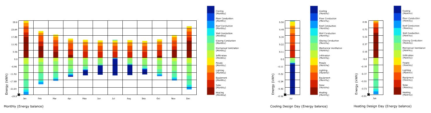
Below is the Energy Balance for the Cooling Design Day and Heating Design day compared to Monthly:
In this way, the pie-chart visualization I’m showing below would essentially be a compilation of three energy modeling runs:
Annual Energy simulation (gives me EUI and total energy use breakdown in the center)
Heating design day for analysis period (gives me a representational breakdown of heat loss components)
Cooling design day for analysis period (gives me a representational breakdown of heat gains)
My overall objective here is to take the information provided in the Monthly Energy Balance a step further by finding a way to visualize how gains/losses connect to end-use heating and cooling energy and resultant building EUI. While these will not be an apples-to-apples correlation in my heating/cooling design day example (because of the different analysis periods), I wonder whether it could be representative of cooling and heating energy contributors, or still too misleading? If a graphic like this is possible, I think it would make more clear to designers the potential that individual optimizations have to directly impact total energy consumption in the context of total building energy use.
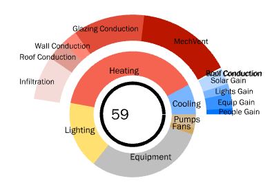
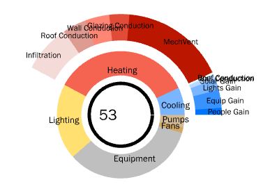
The images below show an example of visualizing the impact of changing WWR ratio from 40% to 10% using the method described above:
A related question on ReadEP Results terms: MechVentilation appears when I am running an Ideal Air Loads model but disappears when I add an HVAC system (VAV w/Reheat). How can I account for OA ventilation gains/losses when I have a specific system added?
For example, if I run the model for the coolingDesignDay to get the breakdown of heat gain components, it seems these results could be proportionally representative of what is contributing most greatly (by %) to cooling energy in general? Similarly, I would then run another simulation on the heatingDesignDay to get a representation of the heat loss breakdown.
The problem is that the design day simulations aren’t proportionally representative of annual energy. It helps to think about this statistically. Design day periods represent the ~0.4%-ile or ~99.6-ile of your annual dry bulb temperatures for cooling and heating respectively[1]. By definition that means it’s a rare event. For Gaussian distributions, anything that is approximately three standard deviations from the mean (0.03%-ile/99.7%-ile) can safely be considered outliers. Another common statistical technique, (for non-Gaussian distributions) is to consider anything outside the 25th and 75th percentiles (the interquartile range) as outliers. Regardless of which technique we use, by definition the design days are not representative of the conditions informing your whole building energy.
My suggestion is to work with the actual constituent data to work out your breakdown, rather then try and map different analysis periods to it. The latter method can lead you astray. When I suggested splitting the analysis into two, I meant something like taking the monthly heat balance, and averaging all the months with mechanical cooling into one breakdown, and averaging all the months with mechanical heating into another. I’ve done that in the past to try and distill the monthly data into a representative heating and cooling season, although this may not work if you have shoulder seasons/moderate climates with simultaneous heating and cooling, so there needs to be way to account for that as well (or just omit it).
A related question on ReadEP Results terms: MechVentilation appears when I am running an Ideal Air Loads model but disappears when I add an HVAC system (VAV w/Reheat). How can I account for OA ventilation gains/losses when I have a specific system added?
The component loads aren’t represented when you model specific systems because the addition of HVAC system efficiencies result in mechanical cooling/heating quantities that are less then the sum of the component loads. So it’s more difficult to conceptually represent your breakdown this way. However you can find and account for different component loads (even if they don’t add up) by looking up different EnergyPlus outputs in the RDD file, and adding it your simulation run as a requested output.
[1] As a general question to the LB community, I’ve always been confused about how ASHRAE defines their percentiles. If you bin your dry bulb temperatures from coolest to warmest temperatures, then by convention the 0.4%-ile should correspond to the colder temperatures, aka your heating design day (reading from left to right). But ASHRAE defines this as the hotter temperatures, which means they’re reading their probability distribution from right to left. What am I missing?