Heat mapping and temperature gradients

Hi. I’ve been using ladybug and honeybee tools for a while now for different kinds of studies. Now, I am pursuing a new study where I am currently encountering a roadblock.

The study is basically an outdoor study on mapping the heat emitted by the building masses at different heights/levels. If possible, it would be great if the result can be isolated from the effects of solar radiation. Basically, we are only visualizing and mapping the temperature gradient of the heat that is being emitted by the building. I am thinking that this is a function of radiant temperature studies.

Kindly let me know if anyone has any ideas on how to go about this. Thank you!

@LanceMonfort,

Honeybee has a component called Read EP Surface Result which contains surface energy data. When you run your simulation, make sure that you use the Generate EP Output component to select surface energy analysis as an output.

If heat is being emitted from the buildings, the energy will be reported as a negative (heat loss).

Forgot to address removing the impact of solar.

For your glass materials, you can subtract the transmitted solar energy from your glass heat transfer, and that should isolate just the conduction contribution of your glass heat transfer. So specifically: glazEnergyFlow - windowTotalSolarEnergy = GlazingConduction.

For the opaque construction, it’s a little trickier since the opaque energy transfer contributed from solar is not isolated and provided in the default results component. There may be a specific output you can call from EnergyPlus for this, but I think you can just ignore the solar contribution completely without huge inaccuracy.

If you have a rainscreen construction, then the energy transfer is occurring from the zone interior to your vented cavity, so that’s already shielded from solar and therefore it doesn’t have any meaningful impact on your heat transfer. If there’s no vented cavity the impact is limited to some thermal lag in the actual opaque construction, but that will be fairly minimal because the insulated assembly will prevent a large temperature deltas to occur.

S

2 Likes

Thank you for your response, Saeran. This is an interesting take on this concern.

Although what I intend to do is visualize the heat being emitted as a colored mesh (very much like a microclimate map) but for something like heat movement. I intend it to be something like a temperature gradient that represents the heat generated by buildings based on their material properties and heat gains.

The take on heat loss from the Read EP Result component is interesting but I’m not sure how I can use that if I want to map values on multiple points in a 3D space to generate my colored mesh.

Do you have any other insights on how this can be done?

@LanceMonfort,

The surface energy in the Read EP Surface Result is the ‘heat movement’. It will represent the change in heat transfer through different levels. If you connect it to the Color Surfaces by EP Result you will have your 3d representation. EnergyPlus is computing the value of the heat transfer at the center point of each surface, so if you want to be more precise, take the center point of each surface, and that collection of points is the computed heat transfer in 3d. If you subdivide the zone exterior surfaces to a greater degree, EnergyPlus will calculate the heat transfer for each of those points and you’ll get a finer gradient to create your mesh. If you do this you will see the gradient you’re looking for, as there’s many changing environmental conditions along that z axis that effect the heat balance: wind, solar, sky view factor etc (although the magnitude of the heat transfer will be minimal through opaque construction).

S

Thanks again for your response, Saeran. That is very insightful.

I gave it a quick try and I was able to map the heat losses and outdoor surface temperature (using a fine grid so it gave a nice gradient) on the surface itself.

That is very interesting but what I was trying to visualize is the heat that is being emanated from the surface. It’s like visualizing radiant heat in 3d space. I’m not actually sure if there is a ladybug/honeybee tool that does exactly this but it would be great if you have any insights or any leads that could help in developing this study?

Kindly let me know. Thank you so much!

Okay maybe we’re getting somewhere now. There are three heat transfer mechanisms: convection, conduction and radiation. You are asking to see just the radiation portion, correct?

In that case what you want is the following formula:

Qrs = a * e * sb * A * (Tsrf^4 - Tenv^4)

where:
Qrs = Radiant energy exchange of a single surface with a surface in it's environment [Wh]
a = absorptivity of your surface [unitless]
e = emissivity of the environment surface [unitless]
sb = Stefan-Boltzman constant [5.67 * 1e-8 W/m2/K^4]
Tsrf = Temperature of your  surface [Kelvin]
Tenv = Temperature of environment viewed by your surface [Kelvin]
A = Surface area [m2]

For a single surface the total radiant exchange will be the sum of the radiant exchange for all surfaces it can “view” multiplied by that view factor.

Qrt = sum(f * Qrs)
where:
Qrt = Total radiant exchange for surface with entire environment
f = view factor for that surface with the corresponding surface it's calculating it's radiant exchange with.

Pretty much everything in these equations you can retrieve from your existing HB model, except the view factor determination which can get kind of tricky, but there is a view factor method in HB to get those. You can also make a simplifying assumption if you have a simple environment. For example if you have a building in the middle of an empty site, you can assume that half the surface is exposed to the sky, and half the surface is exposed to the ground. So your view factor would be 0.5, 0.5 for each, and temperature of environment would be ground surface temperature, and the long-wave temperature of the sky.

Alternatively, there may be some built in method to retrieve radiation energy from the exterior surface, I just can’t think of one right now.

S

1 Like

Thank you so much for that, Saeran!

That is a very interesting lead. I’ll see what I can do with these inputs and let you know of any developments.

Thanks again!

Hi, @SaeranVasanthakumar .

I hope you are well. It’s been a while but I am finally picking up on this again :slight_smile:

I was doing some tests and I have a test model that looks like this:

In the image above, the thermal model is visualized as a red wireframe whereas the test points for the heatmap is visualized as green test points. Let’s say we have 100 surfaces and 500 test points.

Using this formula:

Qrs = a * e * sb * A * (Tsrf^4 - Tenv^4)

The variables a, e, and sb are single values. A and Tsrf are 100 values since they correspond to the surfaces that will be radiating the heat energy.

My question now is: does Tenv correspond to the 500 test points? If so, does this mean our value for Qrs will be some sort of matrix of around 50,000 values which represents the relationship of each surface with each test point? In a way, each of the 100 surfaces will be calculated with each of the test points so that will give us a total of 50,000 values in total.

Is my understanding of this correct? Kindly let me know your thoughts on this. Thank you!

@LanceMonfort

Apologies for my late response. To answer your question:

Technically you are defining 100 a, e, and A (thermal absorptance, emittance, and area) values, since they are specified per surface. You define them when assigning a HB Material to a HB Surface. Typically the surface a = e at the same temperature so you only need to assign one. Obviously if the surfaces are of the same material, you only need to define its thermal absorptance once.

EnergyPlus provides a single measurement of surface temperature per surface, per simulation time. So if you are getting hourly results from your EP simulation, an annual simulation with 8760 hours will result in a 100 x 8760 Tsrf matrix (or 876,000 values in total).

So where do the 500 test points come in? They will vary per surface view factor f (the second part of the equation in my previous post). This is where things get complicated. Each test point has a unique f calculated to all other surfaces in the scene. So if you have 100 surfaces with 1 test point, then each surface must calculate 99 view factors to describe it’s relationship to the other surfaces, or 100 x 99 f values in total. Assuming the 500 test points still just represents one surface with approximately equal temperature (and not 500 subsurface patches), this means each test point must compute 99 view factors, or 500 x 99 x 100 view factors in total. Simplifying 99 to 100 for cleaner math, that gives us 5,000,000 view factors (assuming I didn’t mess up my math anywhere). Luckily this won’t change per time step and only has to be calculated once.

The result sums the 99 other view factors to a single value, so the resulting Qrt value is, as you say, 50,000 points per time step, or a 50,000 x 8760 matrix.

Anyway, the good news you don’t have to do these calculations manually. Its good to get a sense of the underlying theory and intuition for why increasing the number of test points scales computation time quadratically, but in terms of application, LB will do the complicated stuff.

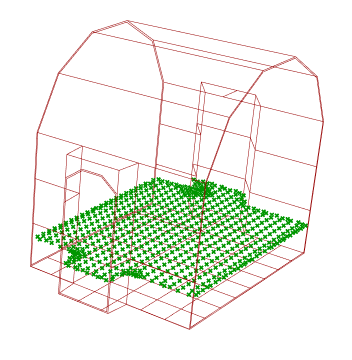
Here’s an (HB Legacy) example that loads surface temperatures from EP, and multiplies it with view factors per test point for a given surface. In this particular case the output is mean radiant temperature (MRT), which is not exactly what you are asking, but is in fact related, and the workflow illustrates the view factor/EP surface temp workflow you need. There is an equivalent (and much improved) version of this with the latest HB, but I don’t have time to search it out now. I’ll try and get back to this discussion when I have more time if you can’t locate it.