I have been trying to run a UTCI study with 2 methods:
a simple one using LB, using wind speeds from the epw file
a more complex one based on HB for surface temperatures.
While it is understood that the former method does not allow, per se, to calculate surface temperatures, the latter has the potential to do so, with a limited number of choices provided in the component HB Ground.
The limitation I am finding with the HB route has to do with the results reporting. I am most certainly using components wrongly, however when I try to extract results using the HB Read Thermal Matrix.
I seem to obtain average values, which do not help showing the behaviour of different materials over time, and quantify the impact of albedo on surface temperatures and ultimately the UHI effect.
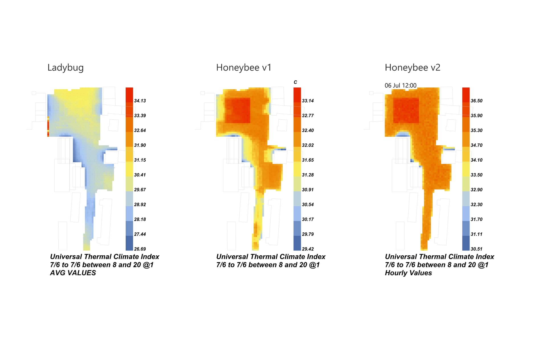
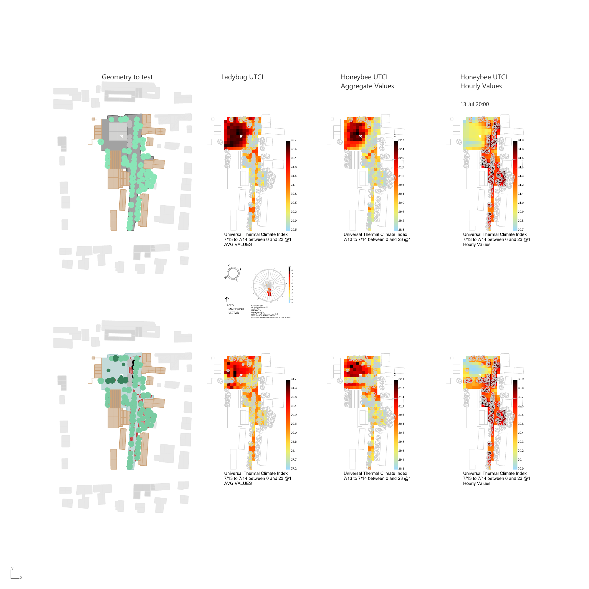
The model is of a public square, and includes shading from surrounding buildings, a central square with concrete paving (visible as a red square) and asphalt all around it. The study was run 8:00-20:00 for one of the warmest days of the climate year.
I am pasting an example comparison beween the values I obtain with:
ladybug
honeybee with aggregate (default) results
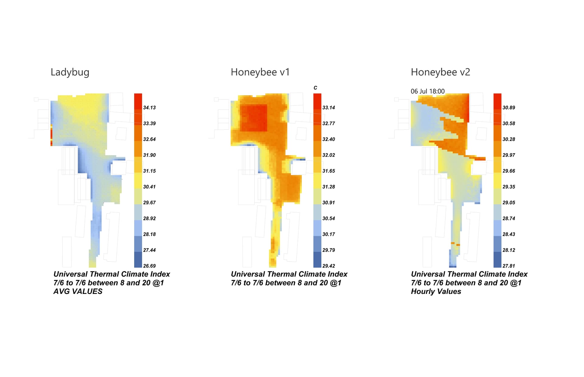
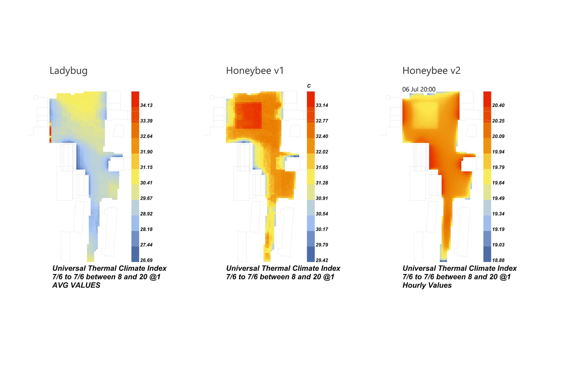
honeybee, with manual results extraction and hourly results
Does that make sense? And why would the typical workflow lead to display aggregate values for the entire run period - hence ‘losing’ the thermal lag / evening UHI effect?
I’ve been meaning to set up a script to share with you to share my approach and see if that helps answer your questions but got distracted by other things - is that something that you’d be interested in?
The results make sense to me. It looks like the higher albedo concrete results in more shortwave energy being reflected upwards towards the human subjects during the daytime, thereby causing a warmer temperature above them compared to the darker asphalt.
This brings up an important point that the Honeybee thermal maps not only account for surface temperatures but also they also account for the shortwave reflectance of these surfaces. In the Ladybug workflow, there are no shortwave solar reflections.
In any event, if you are interested in the UHI effect and thermal lag, then why are you studying the conditions during the daytime when the UHI effect is largely nonexistent? Thermal lag an UHI is going to be most intense immediately after sunset. Also, have you seen these workflows for morphing the input EPW to account for the UHI effect like so?
@chris ,
I have furthered the study and I am even more confused than before.
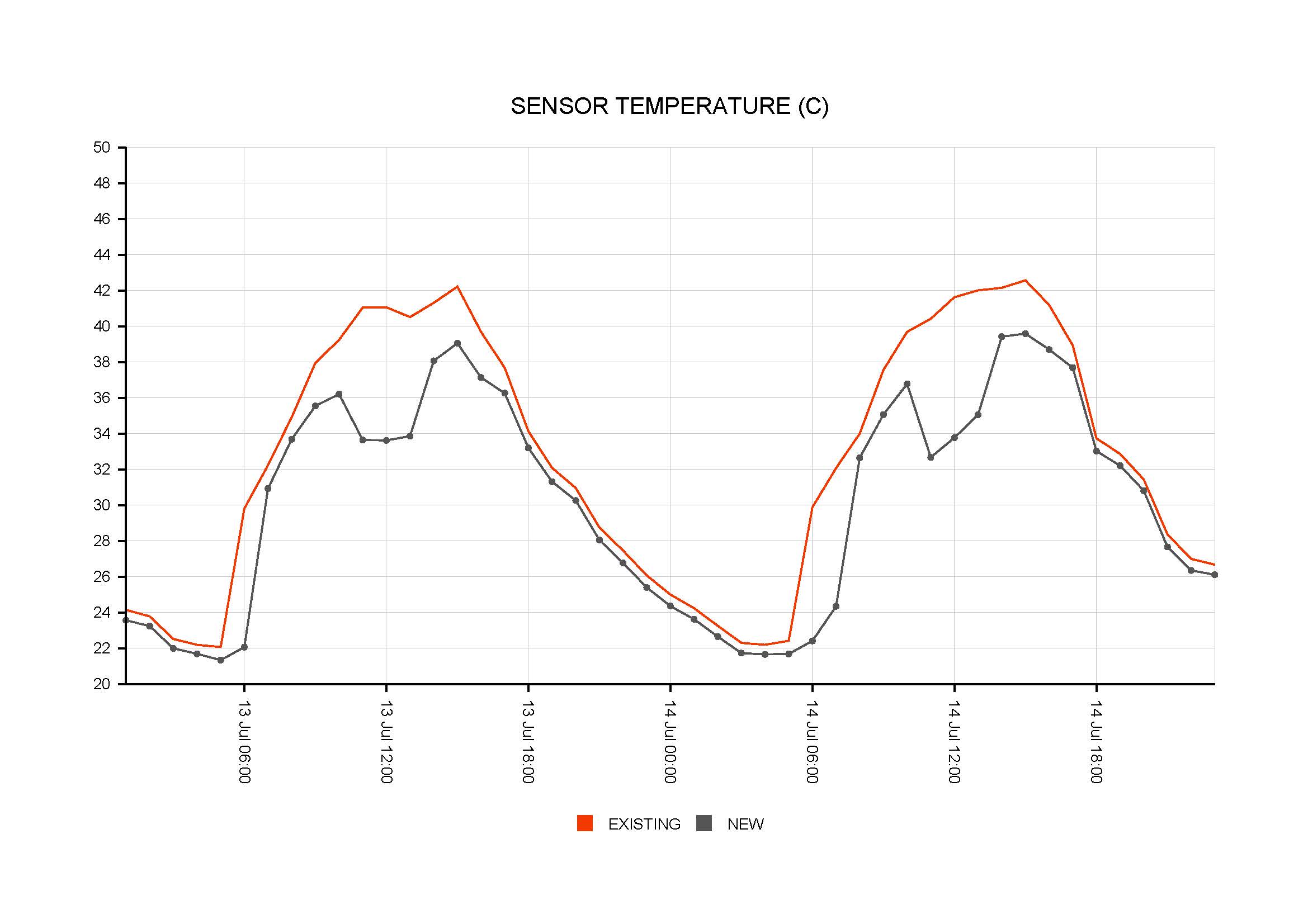
The new UTCI iteration was run for 2 full days - at the start of the hottest week as per stat file - and compared before/after scenarios.
Existing (top) scenario has stone pavement (HB ground material: concrete) and road (material: asphalt) around it. Proposed (bottom) scenario has HB ground mat: Grassy Lawn (I updated to v1.5 to get it!).
UTCI Grid was set at 5m (to shorten calc time) and placed at 2m from the ground.
For both scenarios I have considered a constant wind speed (2.5m/s) which was calculated as an average from epw data during the considered period (48hrs). No CFD data was used for this, for the sake of simplicity.
Temperature difference in the evening (I appreciate and obviously agree with you that UHI most pronounced for a few hours after sunset) is risible, and most pronounced during the day.
This is contradicting everything I thought I knew about thermal lag and UHI !!
Sensor temperature (flagged in white in plans) - appears to be affected only at daytime and due to the shading provided by the additional trees.
It is also curious that the evening temperatures appear to be higher under the trees (modelled as shading elements only) than where the view of the sky is unobstructed (presumably this would be due to obstructions slowing down the release of heat back into the atmosphere?)
I’ve been playing around with the analysis a bit to try and work out how we can present the inputs and outputs in a way that answers your questions most clearly, but haven’t quite got something nice together yet.
I’d recommend looking at what your inputs are and thinking about how that impacts the UTCI calc (air temp, MRT, wind speed, and RH). In the HB UTCI Map process the key aspects are solar radiation and surface temperatures.
Radiation is handled by Radiance, which takes into account reflectances etc.
Surface temperatures are handled by EnergyPlus, taking into account surface temperatures impacted by solar exposure, ground temp, and air temp.
Air temperature, wind speed, and RH all come straight from the weather file (unless otherwise adjusted separately) and so the HB UTCI Map output doesn’t account for any local variations in this.
In your example, I would compare the solar reflectances (both for in EnergyPlus and Radiance) for the materials being simulated in your different scenarios, as well as the thermal mass (and other thermal properties) of the ground material. The differences in these should explain the differences in your results between scenarios.
Because HB UTCI Map is mainly accounting for solar effects (solar exposure of people and surfaces), this is the main difference you’ll see in results.
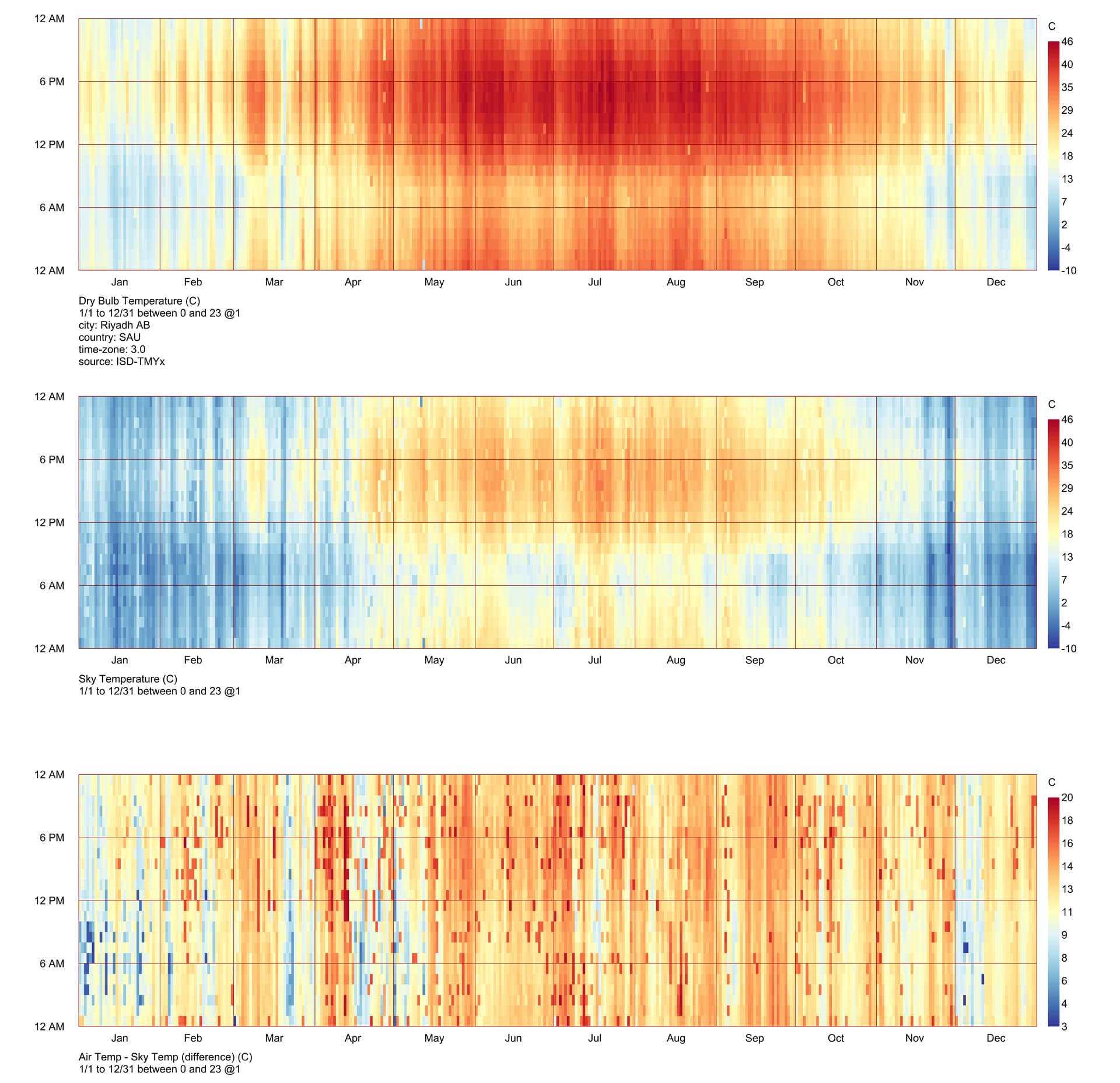
Temperature under trees as simulated by HB UTCI Map will be higher than a similar exposed condition due to sky cooling effect (particularly for clear skies) - the MRT experienced will be higher under a tree where the “shade” above is effectively modelled as equal to air temperature, whereas sky temperature is often much lower. Here’s a comparison of air temperature and sky temperature for Riyadh to demonstrate.

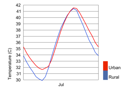