I am trying to simulate a building as an aggregation of shoeboxes to increase the resolution of the analysis for cooling, heating, and lighting demand. In doing so I have encountered some strange results on flat walls that should be providing uniform energy demands.
One case study I am working on is basically a box oriented on the North axis with a curved alcove cut out of it. For some reason I keep getting spikes on certain parts of the flat facades. The climate for this case study is in Canada, Calgary.
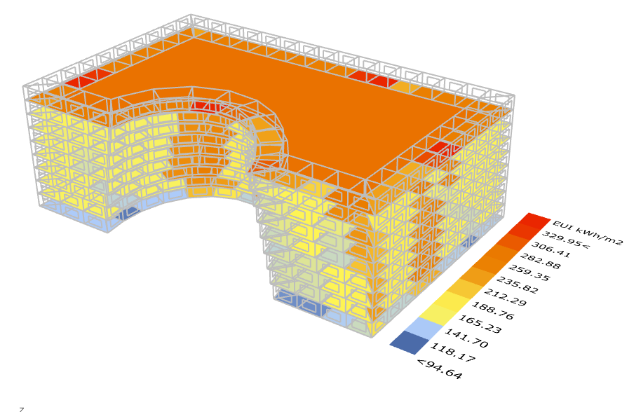
Here you can see on the East side (closest to the legend) for the total EUI a row of much higher demand than the rest of that façade. There is also a couple of shoeboxes that show a dip in demand in blue right next to the row of high demand.
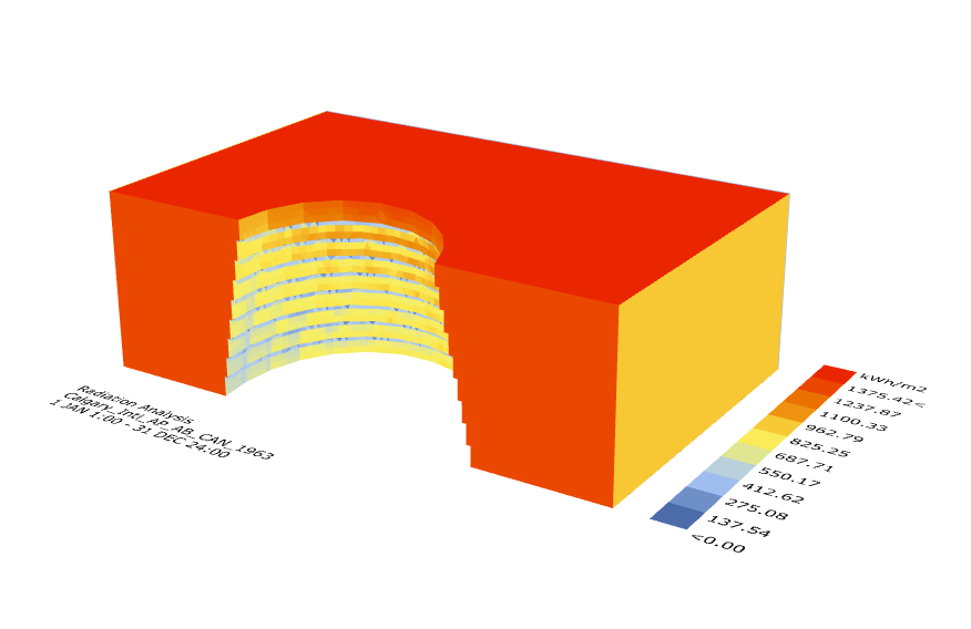
I have compared this to a radiation analysis with Ladybug to check if this was being caused by the difference in solar exposure.
But, from that analysis, I found that the East facing façade had uniform radiation results along the whole façade.
I have tested this setup with various interior wall strategies (Airwall, adjacent, and Adiabatic) and all have yielded consistent results with a row of higher demand.
Has anyone else experienced similar spikes in energy demand results when simulating large facades?
Or is my expectation that a flat façade oriented towards a cardinal direction should produce uniform results across the façade a wrong assumption?
Would very much appreciate people’s opinion on this.
If these zones are all identical (loads, schedules, materials etc), then I agree it’s odd. But this should be easy to debug with Honeybee’s visualization tools.
First, when you build models of this scale, the chances of geometry errors increase to near certainty. So if you haven’t already, I would check the results of visualizing the boundary surfaces, and surface types.
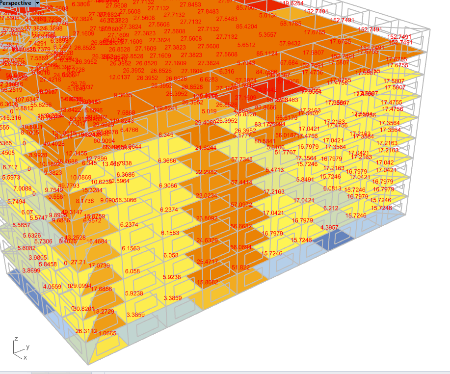
Can you also show the results of the different load breakdowns for each zone? I.e pass the cooling loads, heating loads, window transmitted solar (etc etc) separately in the Color Zones component until you find one that fits the ~50 kWh/m2 difference between adjacent zones.
This is the cooling load. (sorry for how it is visualized, I couldn’t figure out another method to visualize the corresponding data to the shoebox and have opted for putting the value in the center of the shoebox.)
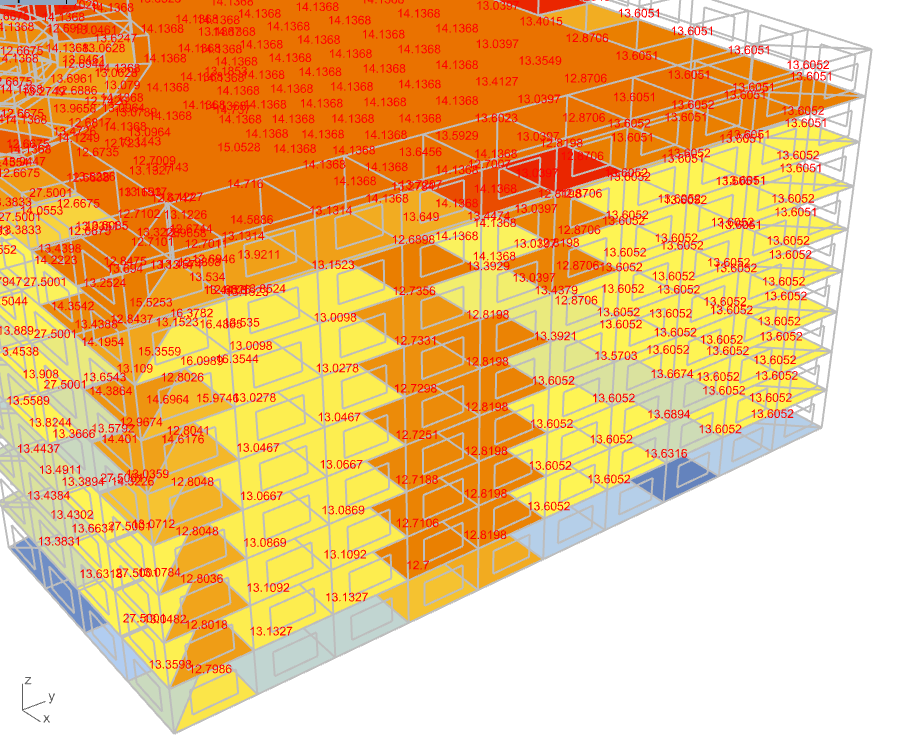
From the breakdown it seems that the EUI difference is being made from a combination of cooling, heating, and lighting loads. Most significantly the cooling load.
Is this perhaps pointing to an error in the way my cooling is being calculated/setup?
If you are running an ideal air loads simulation, take a look at the energy balance workflow for an example of how to get a broader load breakdown, and which loads to investigate. Now you know the mechanical cooling/heating systems are causing the difference (as opposed to electric/lighting use), so try and figure out what is causing the need for mechanical conditioning. For example, is it solar gains, conductive transfer, internal gains from occupants/electric equipment, ventilation etc? Opaque and glazing heat transfer seem likely candidates since you have both higher heating and cooling loads.
You can pass the individual loads in the zone color component that you’re using to visualize the EUI.
Also I’m a little confused by why your lighting load is different if your space types are the same, but I suppose it could just be a result minor numerical inaccuracy caused when processing the EP outputs.
Finally, apologies if you already know this, but there’s two components in the first tab of Honeybee (tab #0, I think) called something like Decompose by Type and Decompose by Boundary Conditions, which will allow you to visualize what you have set for those parameters, which will be the most reliable way to check your input accuracy.
Actually, one more obvious check: are you splitting the faces of the adjacent zone faces so that there’s a 1:1 ratio between matching zone area surfaces?
I’m not sure what your core zones look like, but if it’s one monolithic zone, without the surface adjacent to your perimeter zones subdivided, then that could explain the imbalance. Specifically, the core zone will try and match one of the perimeter zones as it’s adjacency, and then (in accordance with law of conservation) model the entire heat balance between interior and perimeter zones just for that single zone.
Thank you so much Saeran! A lot of great points that I’ll be looking into.
I’ll be sure to post back once I find out what’s been causing the weird results.
After some testing the most likely culprit seems to have been the 1:1 adjacency.
It looked like when I was creating the core zone, the planar surface I was extruding with was simplifying the curve and removing all the knots so it was extruding single faces instead of the multiple it should have been.