Hello, this topic continues my first post on solar radiation and urban large scenes. I would like to share my findings, refine my scope and get any comments. This is definitely a long-read. So, my aim was to process the city scale in one batch, accumulate useful tips and test limits of LB Incident Radiation somehow.
Cases with LBT at the city scale are rare in research papers (I would say there is no such cases). ArcGIS, Simstadt, r.sun and others are quite popular, but not the LBT. So that was a starting point for me.
You can find the conclusions at the end.
The study is conducted using two computer configurations:
- PC1 – i7-7700, RAM 32 GB 2133 MHz, GTX GeForce 1050 Ti, SSD;
- PC2 – i7-13700F, RAM 128 GB 4000MHz, RTX GeForce 4070, SSD (I have just bought this PC a month ago)
Workflow
Preprocessing of geodata
Initial data consist of 2D building footprints, terrain is stored in raster format. I relocated all geometry closer to 0,0,0 and simplified 2D contours to eliminate edges under 1 m. It is easier to do in QGIS compared to Grasshopper.
After importing and extruding contours in Heron, I generated a mesh for each building and baked all geometry to Rhino. Thus I reduce steps in Grasshopper.
TMY
For Sofia, Bulgaria, I used TMY data from OneBuilding, which seems to overlook terrain shading. PVGIS looks more interesting but I didn’t managed to exclude shading caused by surrounding mountains, as it shows the same values for both situations.
Effective shading terrain surface and 3D terrain generation
Yes, Gizmo can be utilized as well but, from my point of view, it is not useful for large area. So I decided to calculate viewsheds in QGIS from key points on the city boundary. The points represent possible skyscrapers and enhance shading area of the terrain. Using the resulting boundary I cropped the coarse terrain mesh.
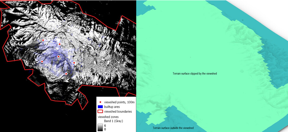
The final mesh terrain was inserted into Rhino.
Cumulative sky and Ladybug Incident Radiation
I chose Incident Radiation instead of Honeybee, because it is easier to manage, but the results can be less precise. I would appreciate any links to such a comparison between IR and Honeybee. In my case I do not have materials for the surroundings and I can’t rely on too rough assumptions. So I choose LB Incident Radiation.
A key feature here is the cumulative sky matrix. The Radiance’s gendaymtx function is used to calculate the radiation value, based on weather data, for each patch of the sky.
If I get it right, a precalculated sky matrix accumulates solar radiation and this significantly reduces the time needed for calculations. Roughly speaking, the only thing you need is to add a shading mask. As a result, there is almost no difference between calculating a full year of 8760 hours or just a single day. But you can’t get the dynamics of shading: it is unknown, when and for how long a face is shaded.
Resolution of study meshes, sky subdivision and context meshes
At this stage I tested the maximum number of faces and sky divisions for stable calculations in case of PC1.
Here are the results.
| cell size, m | face count | Tregenza sky, sec | T, with shade 446984 faces | Reinhart sky, sec | Reinhart sky, sec, grafted | Tregenza sky, PC2, sec |
|---|---|---|---|---|---|---|
| 3 | 35931 | 22.5 | 22.6 | 84 | 84 | 17.6 |
| 2 | 78806 | 30 | 49.6 | 180 | 186 | 35.8 |
| 1 | 321574 | 198 | 198 | 840 | 804 | 180 |
| 0.75 | 568692 | 372 | 354 | 2400 | 2016 | 228 |
| 0.5 | 1286308 | 798 | 834 | - | - | 528 |
| 0.4 | 1988897 | 2376 | - | - | - | 876 |
| 0.25 | 5146622 | 33480 | - | - | - | 2394 |
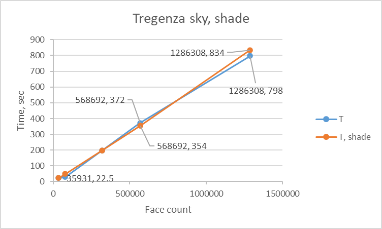
The chart for PC1 is displayed below. After 2 million faces, the time cost begins to increase exponentially and the application starts freezing frequently. As for PC2, it goes fine with 5 million faces.

To ensure stability of calculation a study with 5146622 faces used a scaled model with 1 meter size of a grid instead of 0.25 meter (as it seemed to me).
The Reinhart sky subdivision seems to make a calculation 4 times longer.
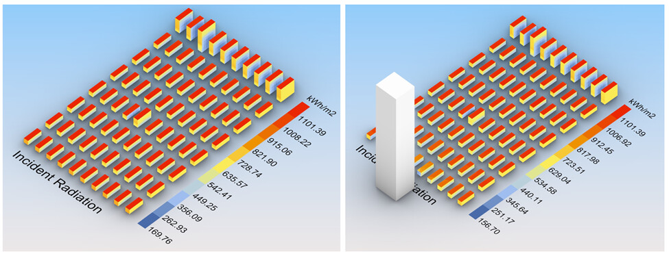
Another point is related to the density of a shading mesh. Shading geometry can be added separately in LB Incident Radiation component. The chart below shows that there is no significant impact of a shading mesh with 446984 faces on calculation time.
Distant shading objects
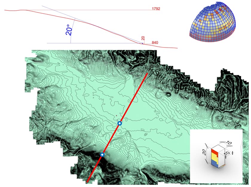
Do we need to model surrounding mountains from the south? In case of Sofia, there is no strong need for that if you are working with the central part of the city. I evaluated horizontal and vertical faces. If your building sits very close to the steep slope, it will produce a certain impact on radiation values for vertical faces for sure. A schematic section for two test points is shown below.
Horizontal faces
| total kWh, y | shading from SW | percentage | |
|---|---|---|---|
| 1- no shading at all | 145570.0877 | no | 100.00% |
| 2 - close to the slope | 141928.7915 | yes | 97.50% |
Vertical faces
| total kWh, y | shading from SW | percentage | |
|---|---|---|---|
| 1 - no shading at all + plane blocking grnd refl | 231873.0974 | no | 100.00% |
| 2 - close to the slope | 195235.4617 | yes | 84.20% |
| 3 - city center | 221454.6975 | yes | 95.51% |
Maybe a super steep slope will produce more dramatic results.
The terrain mesh consists of ~240 000 but there is almost no increase in time.
Sky mask visualization
This step can be useful if you need to estimate how a skyline is represented in calculations. Differences in height up to 10 meters can be negligible even on medium distances. Tregenza sky is less sensitive to complex shading surroundings, and one can recommend using Reinhart sky in this case.
It is interesting that the Tregenza sky has a several shift while being visualized (see this post).
From Rhino to Web GIS
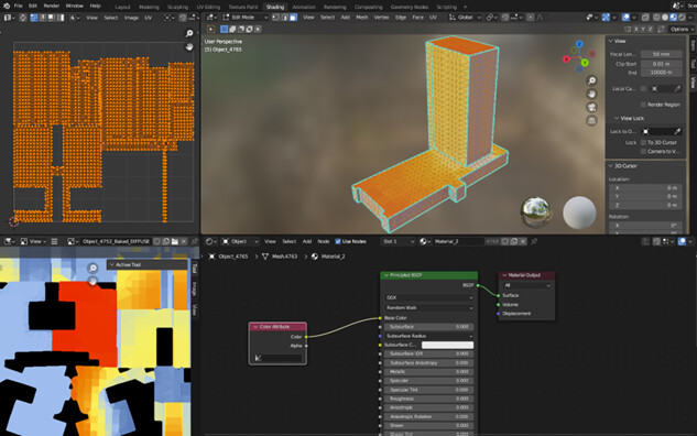
It is a tricky part. We need to visualize somewhere our calculations, and it is better to provide an interactive environment. The only way to upload somewhere large meshes with vertex colors is to bake these colors into textures. This can be done in Grasshopper, but I preferred to use Blender and a modified addon script.
Another issues is related to merged meshes. LB Incident Radiation merges all the meshes after everything is processed. So it is hard to get per-building results (I saw several solutions across the forum). I used grafted study meshes as input, but it increased the time cost too much.
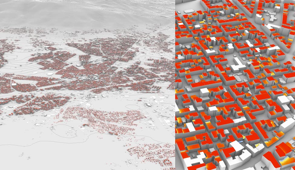
City scale
The first case considers the whole city of Sofia. It is around 150 000 buildings (meshed with minimum number of triangles for shading purposes) and a large terrain mesh. However, study meshes were reduced. Only 64379 rooftops from ~150 000 of residential buildings were selected for the analysis, roofs are flat. Footprints with area below 20 sq.m. were excluded. The conversion of boundary representation objects into meshes with 3-meter edge length led to 1909499 faces. Tregenza subdivion.
| cellsize | faces | PC1, sec | PC2, sec |
|---|---|---|---|
| 3m | 1909499 | 1926 | 1536 |
| 2m | 3698725 | 10300 | 3300 |
Exporting of rooftops to geodata is almost obvious so I skip this step.
District scale
This case goes a bit further with roof details. Footprints from the cadastral map were subdivided into parts according to height differences coming from raster data. The initial DSM from a photogrammetric survey was divided into height-based groups using the Segment Mean Shift algorithm in ArcGIS Pro.
Then I calculated yearly radiation values. Tregenza subdivision, shading terrain is included.

Grafting was used to get per-building results and to merge them with textured meshes in 3D GIS. I would consider to use another approach, because it is a real headache.
So, results are as follows:
| cellsize | faces | grafted | PC1, sec | PC2, sec |
|---|---|---|---|---|
| 3m | 10008585 | no | 684 | tbc |
| 3m | 10008585 | yes | 28080 | 13320 |
Then colored meshes were exported to Blender, vertex colors were baked to textures and the initial meshes were decimated.
The usage of the export of building centroids via Heron (should be merged with textured meshes)

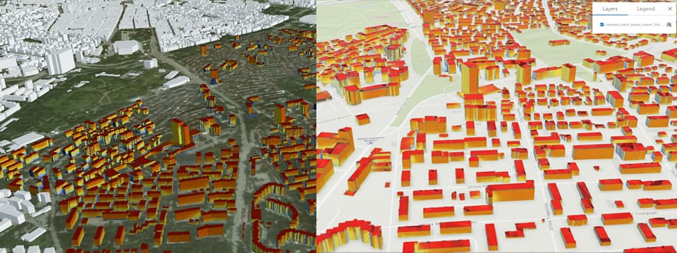
To prepare these data for 3D GIS, resulting geometry was processed with FME and exported to ArcGIS Pro for further sharing of a slpk file. The fbx is deaggregated, relocated to the right position.
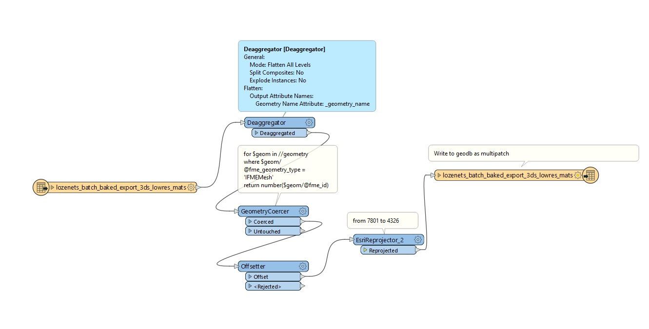
Finally, I got textured lowpoly buildings in ArcGIS Online and Cesium. There is still room for optimization.
Comparison to calculation of solar radiation using GIS
Before switching to Ladybug, I have been playing with ArcGIS and solar calculations. My PC1 has been calculating yearly values a raster with ~70 million cells for 24 hours. And ArcGIS uses the Uniform overcast sky and no TMY. I think it will calculate for ages if you apply average monthly radiation for each step.
The Point radiation looks more friendly: only residential buildings (3 m/pt per 64379 buildings = 1909499 points) – 4 hours. I am not sure about sky divisions and other parameters in ArcGIS, but this still a way longer than LB does. In addition, working with 3D is limited and inconvenient.
Settings for ArcGIS
Latitude 42.65321747622578
Sky size / Resolution 200
Time configuration MultiDays 2023 1 365
Day interval 14
Hour interval 1
Create outputs for each interval NOINTERVAL
Z factor 1
Slope and aspect input type FROM_DEM
Calculation directions 32
Zenith divisions 8
Azimuth divisions 8
Diffuse model type UNIFORM_SKY
Diffuse proportion 0.3
Transmittivity 0.5
What did we get as conclusions in case of LB Incident Radiation?
- Preprocessing steps for geodata, sub-meter features to be removed in case of large scenes (can be more tricky when we have 3D buildings - defeature details?)
- Viewsheds for selecting an effective shading surface (can be used to get shading buildings)
- Shading geometry can be quite large for IR; almost no impact on a calculation time; it is easier to assess visually than horizon bands.
- There is no strong impact of distant shading geometry for horizontal faces. Vertical faces are more sensitive for distant shading if located close to steep slopes
- City scale is possible without tiling
- A regular PC does not work well when calculating more than 3 000 000 points. However, no comprehensive study has been conducted.
- RAM seems to be the most valuable resource for large calculations.
- LB IR looks a way more flexible and promising compared to ArcGIS or other GIS
- An assumption: simplified calculation with LB Incident radiation won’t be misleading compared to Honeybee; should be fine for preliminary assessment at the city scale.
Thank you for your time! Any comments appreciated!
UPD: @chris @charlie.brooker I would really value your feedback on it.