Hello,
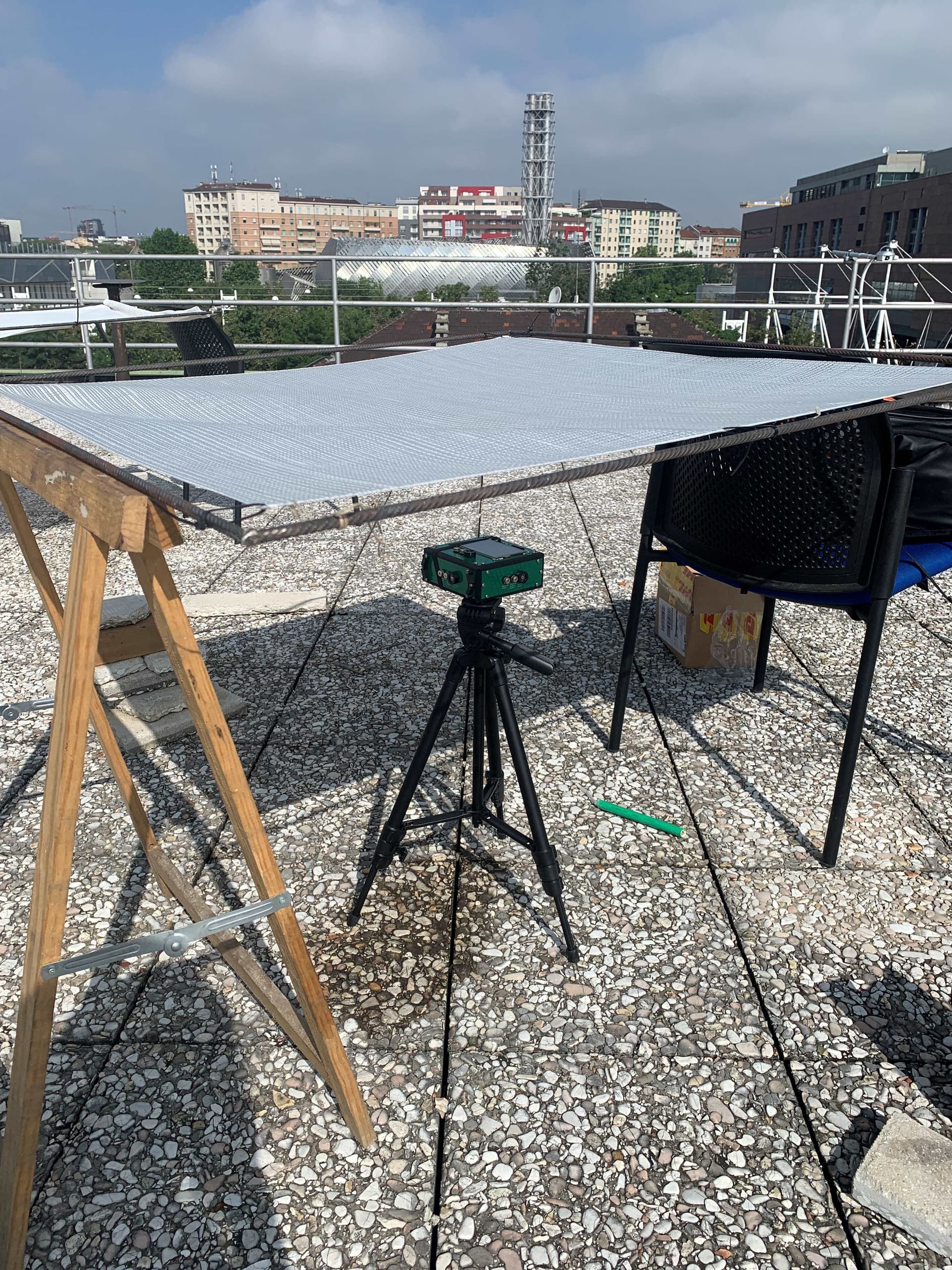
I’m trying to validate Honeybee’s UTCI component swMRT and lwMRT simulations. I have a very simple experimental & model set up with just a 1x1m square piece of shade textile set 80cm above the ground with 6 directional sw and lw sensors approx 60cm above the ground underneath the shade.
Literally this:
I’m trying two modelling options: 1 where the textile is just shade context and reflectivity and transmissivity are set according to the textile properties and option 2 where the shade textile is the roof of a room with open windows.
Either option i use gives very different results depending on the radiance parameters. I read in @chris 's response to this post (Repeating Honeybee Simulation Results in Different Shortwave MRT Delta Everytime - #20 by regwan) to use rfluxmtx | annual for thermal comfort studies, however i get results closer to my measurements with the default settings compared with rflux at any quality.
E.g:
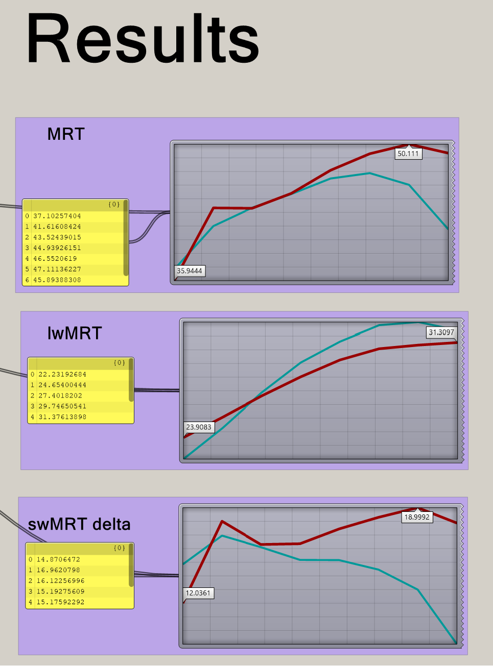
Textile as shade context model
MRT results with default settings
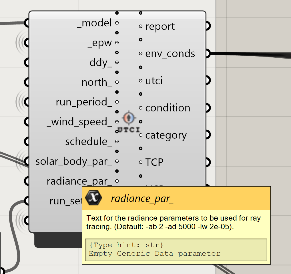
Can you paste exactly what radiance parameters you’re using that you think are “better”? I saw that you originally posted this question under Honeybee[+] (the older version of the current LBT honeybee) and I would want to make sure you are using the right components. The ones that I would be recommending are this one to set up the Radiance Parameters (using the annual recipe type) and this one to run the thermal map that gives you MRT and UTCI. Modeling your textile canopy as a translucent shade is definitely the best way to model it since modeling it as a honeybee Room is going to be opaque and have way more thermal mass than a fabric canopy has.
Also note that the way shortwave MRT is computed in the comfort maps is by using the SolarCal model described in this paper to estimate the MRT delta that would be felt over a human geometry, which is often not the exact thing you are measuring with real experimental setups. So just bear in mind that you may need to tweak your shortwave experimental data if you want it to match what a human experiences and what the comfort maps are computing.
I would expect there to be a better matching of your experimental data with the longwave MRT results, which use spherical view factors in the comfort maps rather than a human geometry. I’m happy to see that this appears to be the case.
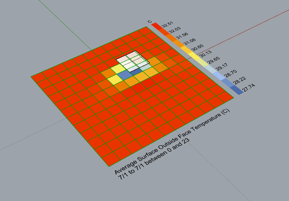
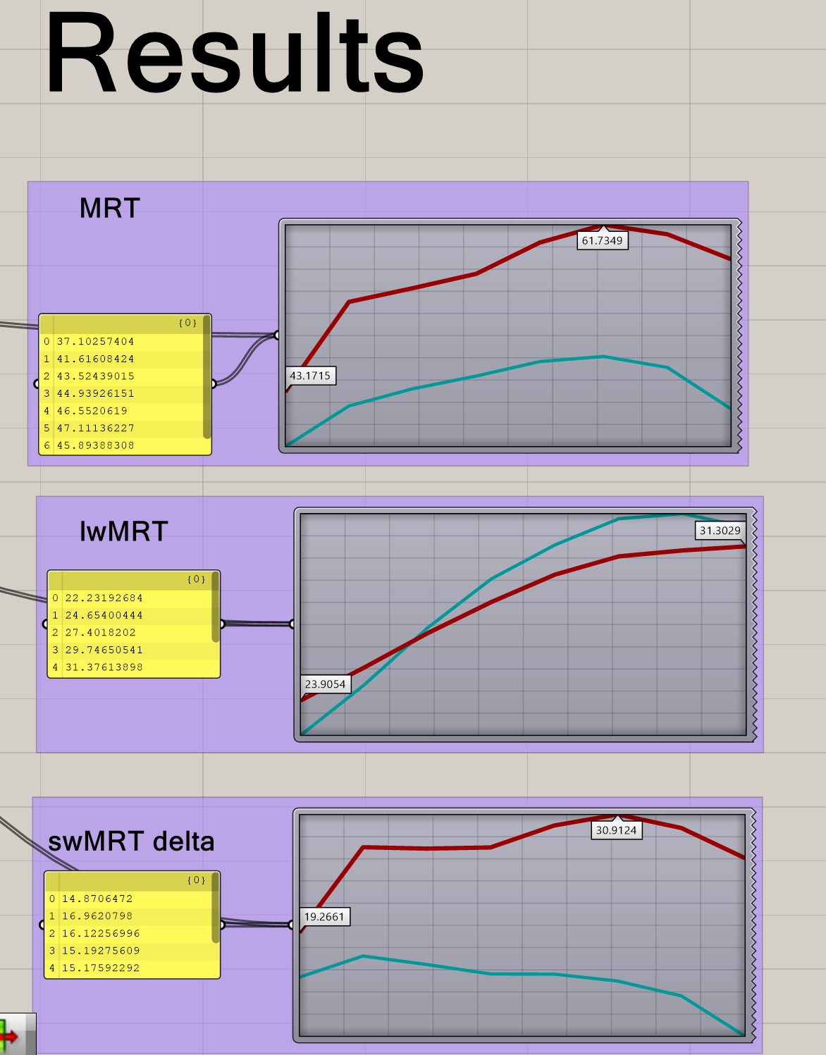
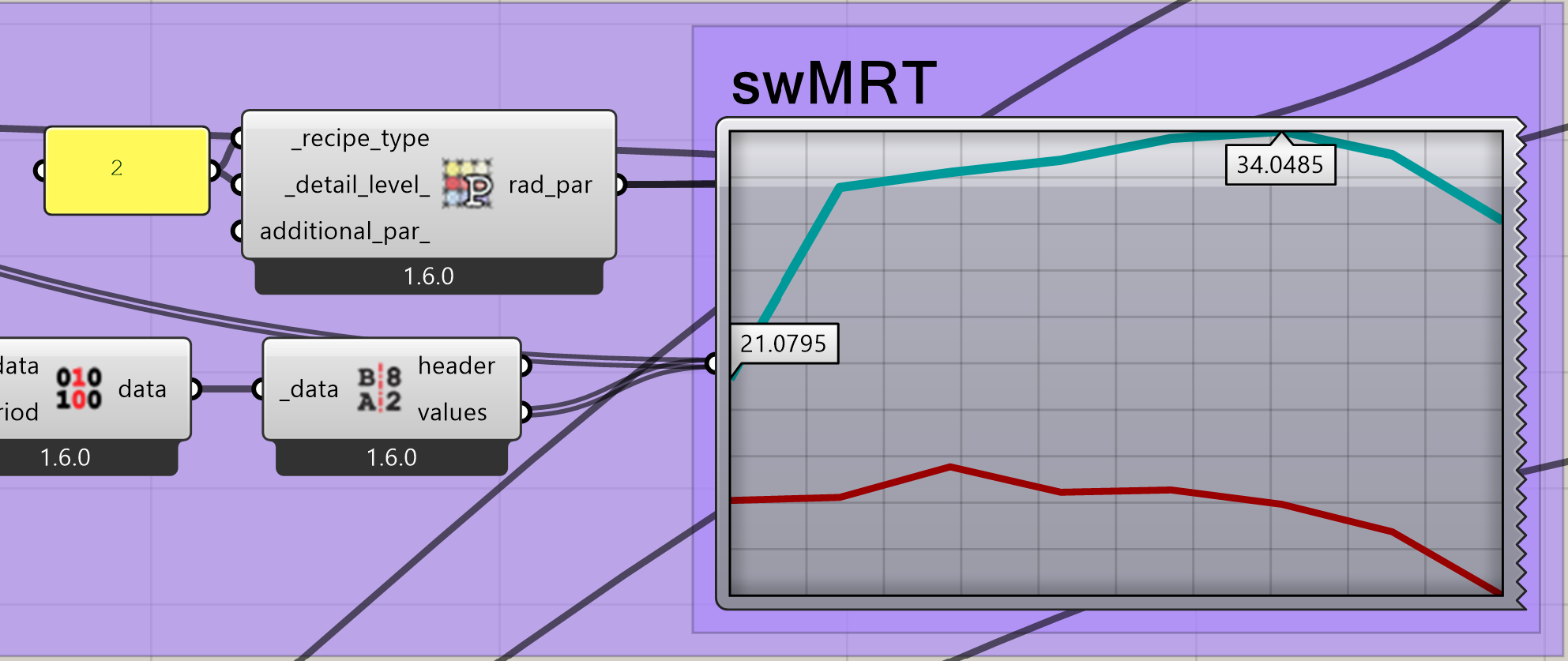
When i use the annual setting, with quality setting as 2 i get way higher shortwave MRT values e.g - this is the sw MRT for the shade as context with the annual radiance params:
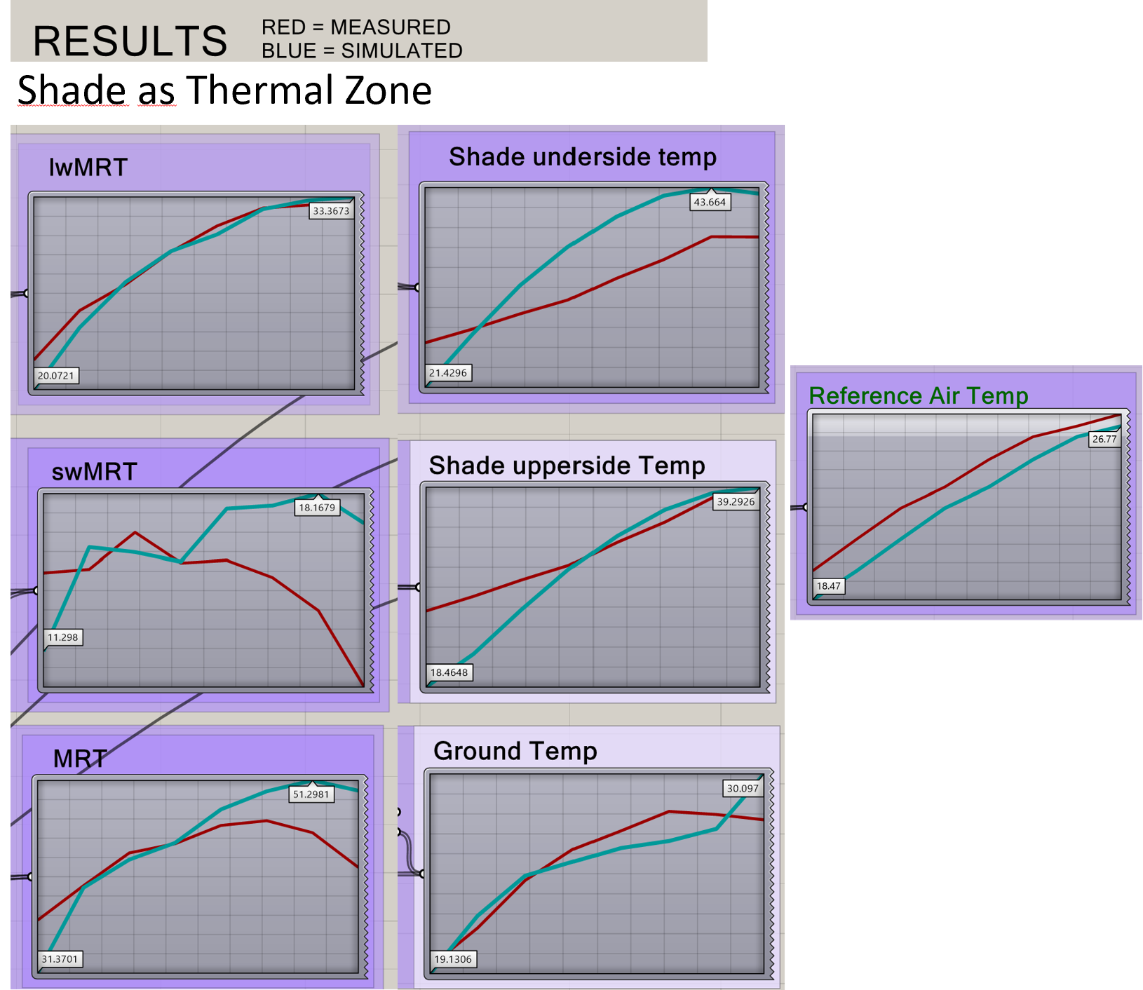
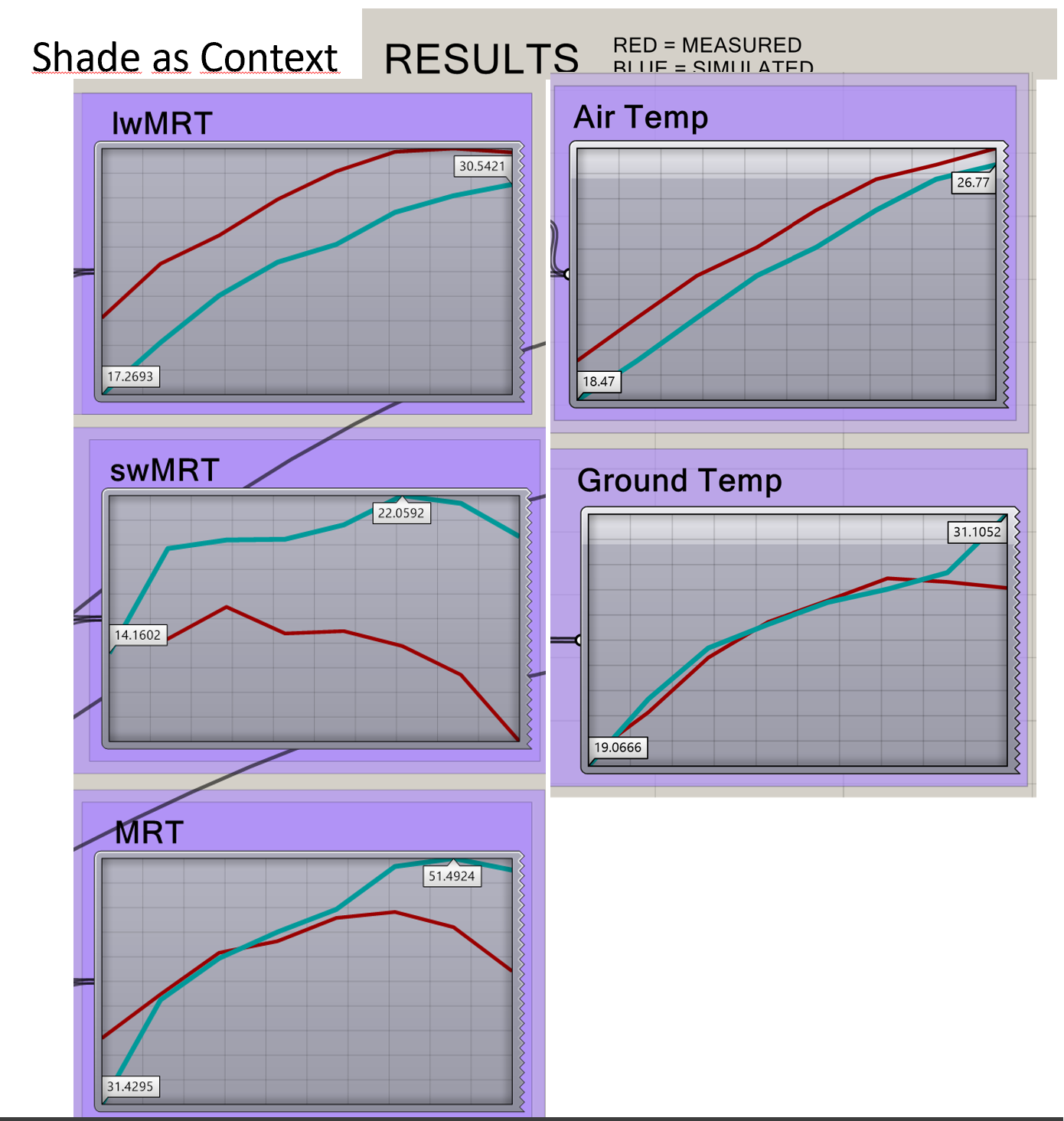
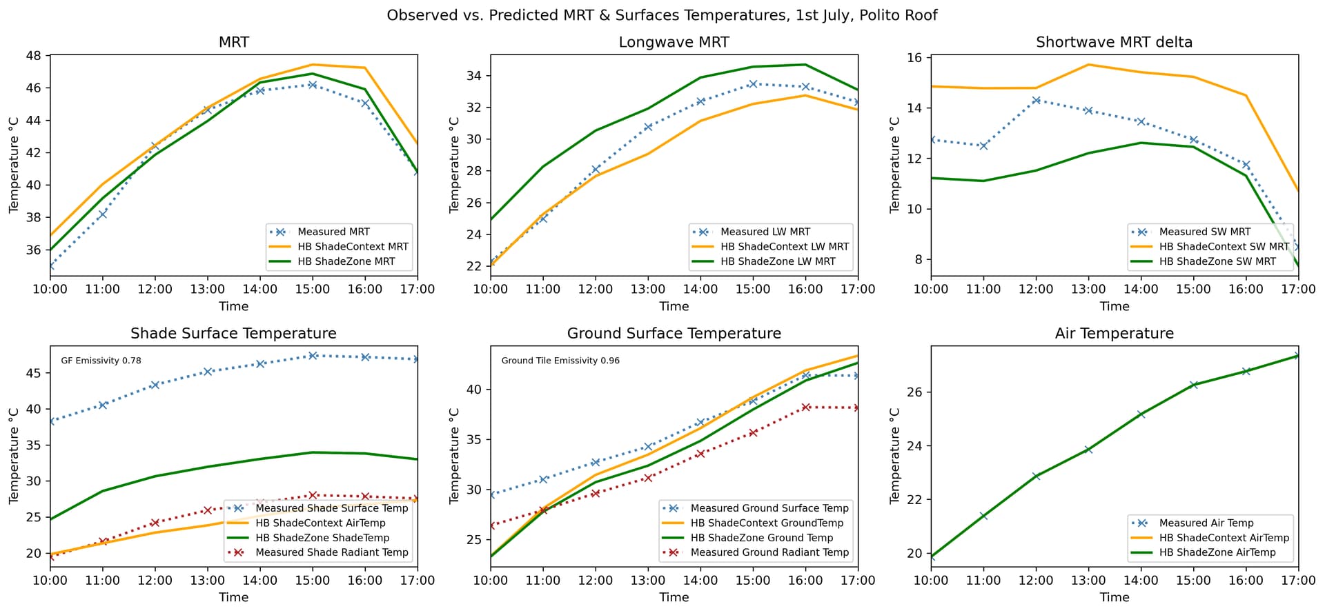
how to model the shade…I have some decent results with the shade as context method, worse results with the shade as room method, and then i tried shade as a very thin thermal zone and HB Opaque Material No Mass which produced the closest results, especially for lw MRT ( ). Here’s the resulting simulated vs measured results for both methods (thin zone vs context)
I think because the material in the experiment is absorbing more solar radiation than a standard shade textile (its glassfibre coated in a plastic resin) its temp is higher than air temp so it is contributing to lw MRT as opposed to the assumptions made when its modelled as HB shade context. I.e that it is same as air temp (and therefore not contributing to lwMRT?). I think you can see in the results when it’s modelled as shade context the lwMRT is lower than in the shade as a zone version.
As for the swMRT, i’m not as on top of this. I would have expected the shade as context model to have more accurate swMRT since i can model the transmittance of the shade but it’s overestimated by up to 10K. I calculated the sw delta from the experimental data with the following equation, using the sw absorption coefficient of 0.7 from the HB default.:
I can see that the SolarCal model is quite different, but haven’t understood yet how to compare with the equation i used. Do you think this could be the main difference in swMRT?
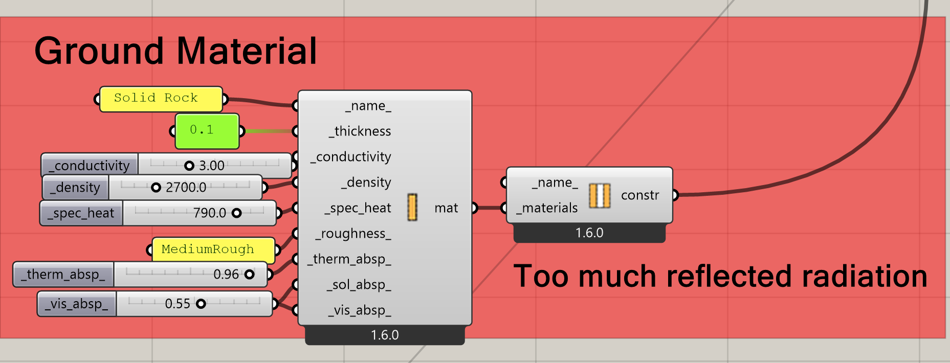
Because also (!) I’m not sure about the ground material properties. Since i don’t know the real material I just went through the list of ground constructions and found Solid Rock gave best ground temp results once i reduced thickness to 0.1. It seems like it’s reflecting too much radiation judging from the swMRT of both but im a bit wary of playing with ground properties too much and getting false results.
These are my ground properties for reference:
-Also would the shade thermal zone be interacting with the ground thermal zone? i.e is too high reflectivity of the ground causing the too high surface temp of the underside of the canopy, or it’s because it’s a thermal zone and storing too much heat?
I think i understand how to calculate the sw delta if i assumed the shade is opaque but i’ll outline the steps here for anyone to check (please!).
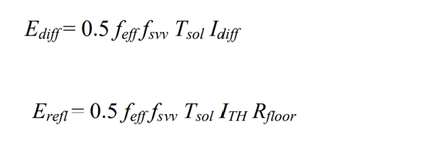
Relevant equations from the paper:
since i have the measured values of radiation after it’s passed through the geometry i can ignore floor reflectance (Rfloor) and Tsol
assuming the shade is opaque i can also ignore direct solar radiation
Which leaves me with s_flux = 0.5 x fract_exposed(fsvv) x posture(feff) x averagedSW radiation (from all 6 directions)
(I would take fract_exposed from LB Human to Sky Relation component (sky exposure output)
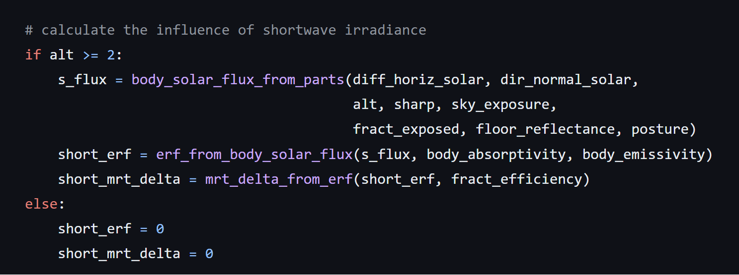
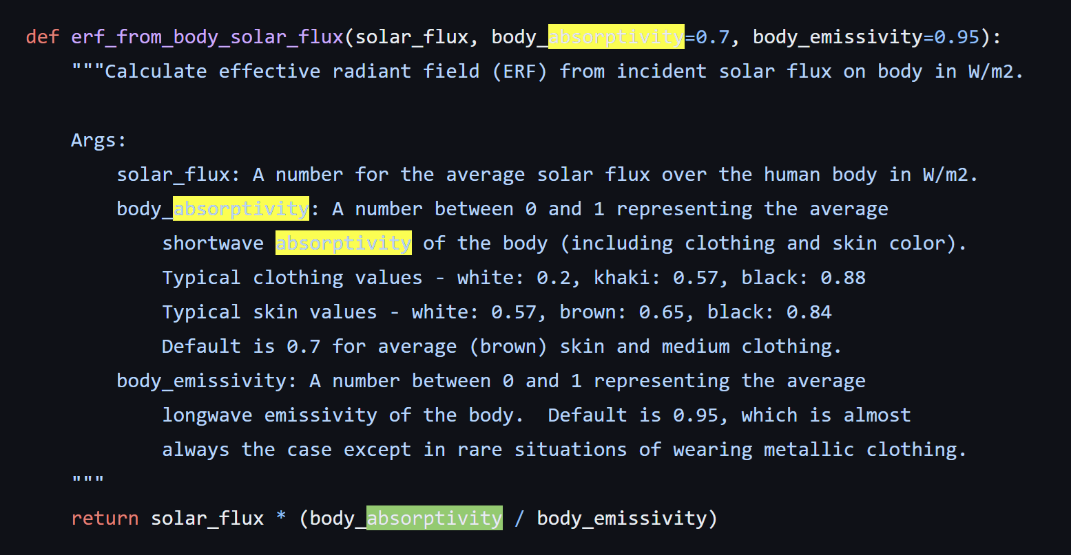
-Then short_erf = s_flux x (body_absorptivity/body_emissivity)
as shown here:
Then mrt_delta = short_erf x fract_efficiency
Why again? I’m not sure i understand this part?
If i wanted to be more accurate and consider that the shade is about 0.1 porous and therefore some direct solar radiation is affecting MRT I guess i would need to:
split the 6 directions and consider the downwards SW measurements as the reflected component, lateral SW measurements as diffuse component and upwards SW measurements as direct component. Using this equation:
multiply diffuse and reflected by 0.5 x posture x fract_exposed
find Ap based on alt and SHARP (fixed at 135°) and projection factor. Is there a simplification for this so i dont have to change altitude for every hour?
take fbes (fraction body exposed to direct sunlight) from LB Human to Sky Exposure Component)
solve Ap/Ad x fbes x direct SW and add to diffuse and reflected SW
But i’m not sure the way im splitting the direction of sensors for direct/diffuse/reflected is correct. I will try the calculation just as opaque and see how it compares
You are right that I would expect a no-mass Room model to give the best estimate of longwave MRT. I guess the most accurate way to simulate the radiant temperatures in your case is to compute longwave MRT using the no-mass Room and shortwave MRT using a transparent shade.
For translating your measurements into a SolarCal MRT Delta, are your sensors effectively pyranometers, which can give you shortwave irradiance values in W/m2? If so, you can plug these values into the LB Solar MRT from Components component to translate them into the shortwave MRT Delta of the SolarCal model that the Comfort Maps are using.
Hi, i do get shortwave irradiance values in W/m2 and tried inputting the sum of the sensors 6 directions as diffuse radiation (direct radiation, lwMRT and ground reflection as 0) but the result is very high. Am i doing something wrong?
That’s great that you can get shortwave W/m2 from the sensors.
To correctly translate your experimental measurements of W/m2 into a SolarCal MRT Delta, you should not be summing all 6 directions. Instead, you would just use the irradiance data from the sensor pointing upwards as the input for the horiz_rad and you can estimate the “ground reflectance” input for that component by dividing the average value of your sensor pointing downwards by the average value of the sensor pointing upwards. If you’re sure that your canopy is diffusing all of the direct sun that reaches your sensor, then plugging the whole W/m2 value into the diffuse radiation is fine. Otherwise, you may want to split this between direct and diffuse if you have any direct/diffuse visual transmittance data about your canopy.
That should give you a shortwave MRT detla that you can compare to the output of the comfort maps (assuming that you have matched the _solar_body_par_ between the comfort map components and the one you are using there to process your experimental results. And you shoudl probably change fract_body_exp_ to 1 to match the assumption of the comfort maps (though that won’t have an impact if all of your shortwave solar is diffuse).
Hello, thanks a lot for the help so far! I made a big edit to this post because I realised I’d flipped north and south measurements.
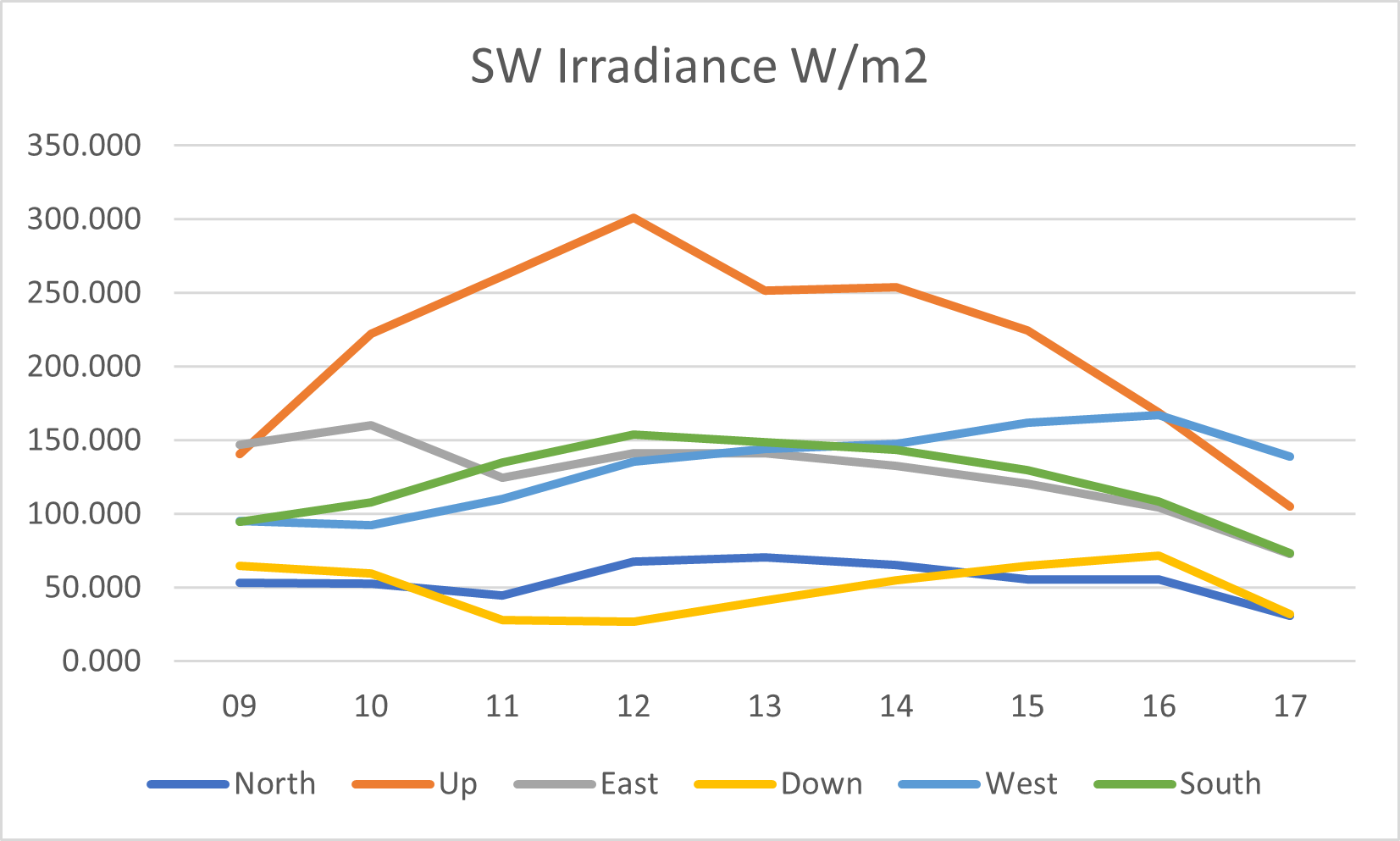
Now results are starting to make a lot more sense! Although I’m not clear about why i would use just the upwards sensor to calculate the delta and estimate the ground reflectivity (from up/down measurements)? Because the sensor (‘human body’) is fairly exposed to irradiance from lateral directions. Here’s what the irradiance data looks like:
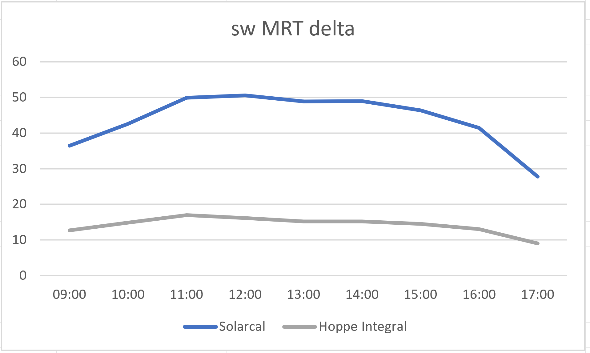
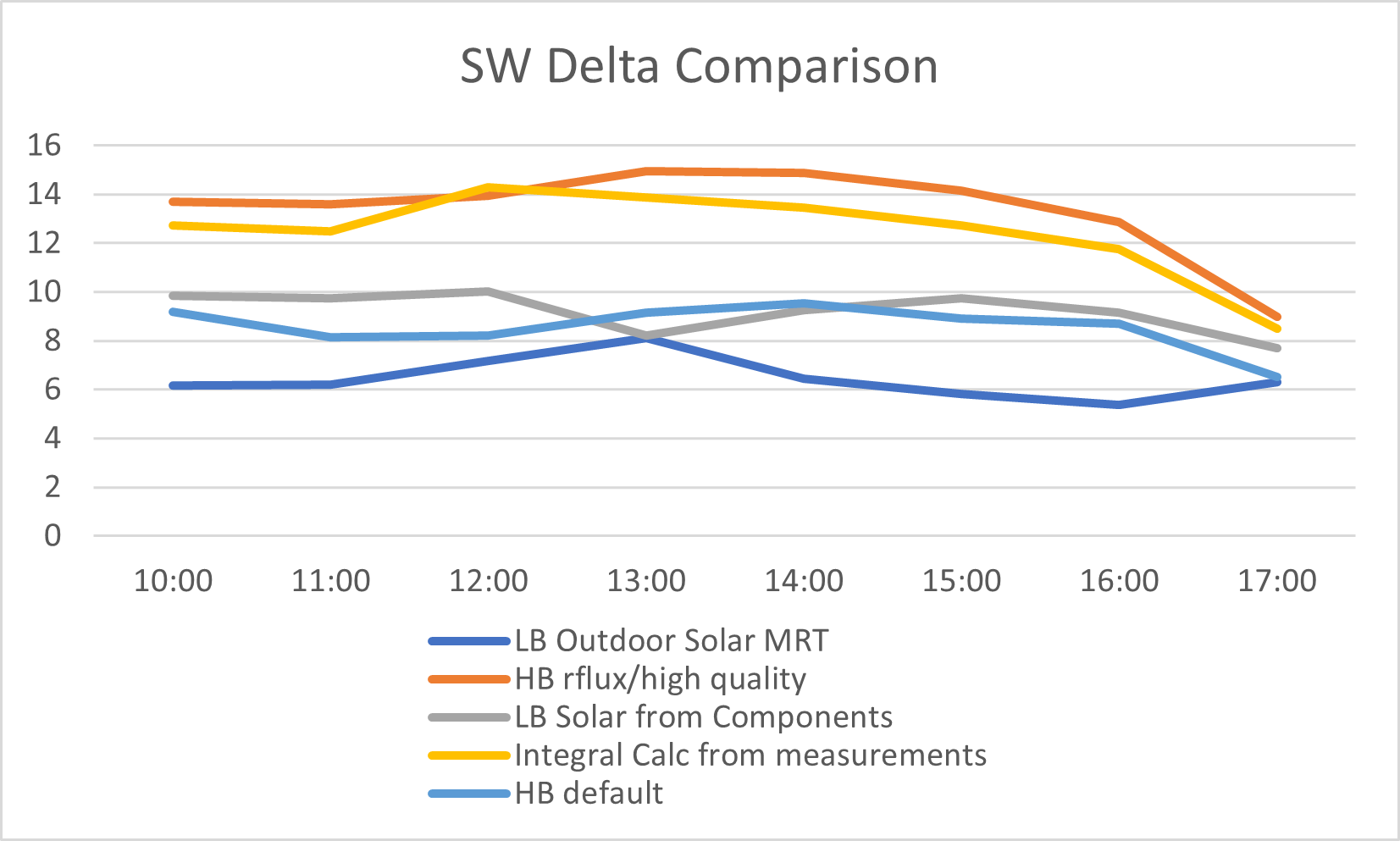
Here are the resulting SW delta’s from HB (with default vs rflux Radiance parameters), LB Solar from Components, LB Outdoor Solar MRT and the calculated SW delta from the integral method. Body params were matched between HB, LB and measurements. And I assumed it’s all diffuse radiation for Solar from Components since i don’t have the material transmittance data.
Following up on this. I have some very good agreement with my field measurements except for the shortwave MRT and shade surface which I explain more below, but in brief I’m wondering if I can improve the sw mrt through radiance parameters and I want to confirm does the UTCI component consider emissivity in the longwave MRT calculation?
SW Delta - I tried different combinations of -ab -ad and -lw after learning from here (Radiance Parameters for Daylight Analysis - #7 by sarith) that these are the 3 most important radiance parameters for the rflux setting. I could only get stable results when -ab was above 5, but the SW MRT was overestimated in both cases, by up to 8C. To get results close to the measured SW MRT i had to limit -ab to 2 but despite trying many combinations of -ad and -lw with it, it still ended up varying by up to 5 degrees between simulation runs. I guess that some of the issue is because i only have one sensor point and so it’s very sensitive to variance but is there anything else i can try to make this more stable? And am i right in thinking that the effect of shortwave radiation is being overestimated either by the way I’ve set the radiance parameters or in the actual calculation of sw mrt? It seems to agree with some other studies i’ve come across e.g Redirecting, Redirecting, Redirecting)
Surface Temps - LW MRT is closest in the shade as context model because it assumes the shade surface is the same as air temperature. The shade’s measured radiant temperature is close to air temperature so this works out in the simulation.
BUT - the shade material has a measured emissivity of 0.78, so when I calculated the actual surface temperature (Stefan-Boltzman’s Law : P/A = є σ T^4), it’s much higher than what is being simulated. When i model the shade as a thermal zone, the temperature was a few degrees higher than the measured radiant temperature as I would expect leading to a higher LW MRT.
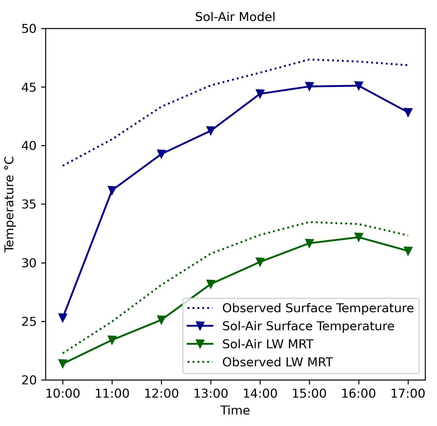
When i did everything manually- calculating the shade surface temperature with the Tsol-air equation and irradiance values and view factors from the UTCI components, the resulting surface temperature is much closer to that measured. Then when i calculated LW MRT manually but including material emissivity values in the equation i get a fairly close LW MRT to that measured also.
So im trying to understand what’s going on - the ShadeContext model works in this case because the radiant temperature of the shade is close to air temperature. The ShadeZone model is a bit overestimated because the simulated surface is a few degrees higher than radiant temp and no emissivity is included in the LW MRT calculation. It kind of works for this case study but if i was modelling a surface with high solar absorption and low emissivity (i.e like some photovoltaics) it would be quite inaccurate. It’s a very specific use case but i’m interested in understanding how i might used LBT to test various ‘non-standard’ lighweight materials like pv’s or radiant cooling materials, and design optimised shade.
Sorry, I have a question regarding the calculation of MRT measured shortwave and longwave separately. I know how to calculate total MRT from Wet-Bulb Globe Temperature but I don’t know how I can calculate swMRT and lwMRT separately. Thank you very much!
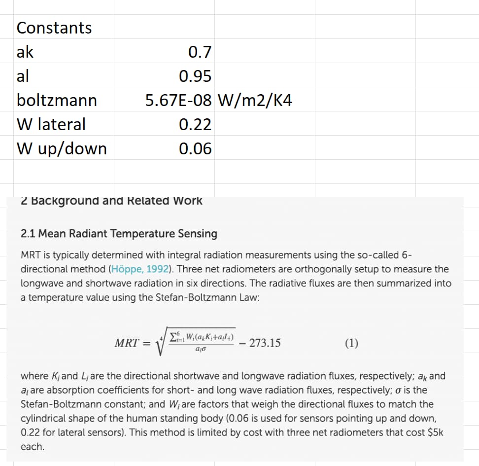
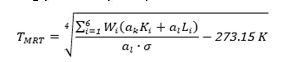
If you are talking about calculating MRT from measurements, you would need to follow the six direction integral method and use sensors that give you both incoming shortwave radiation and longwave radiation. Then you would use an equation like that below to calculate the shortwave and longwave components of MRT (K is the shortwave part, L is the longwave part):
from this paper: Aviv, D., Guo, H., Middel, A., & Meggers, F. (2021). Evaluating radiant heat in an outdoor urban environment: Resolving spatial and temporal variations with two sensing platforms and data-driven simulation. Urban Climate, 35, 100745. Redirecting
You can also predict the shortwave and longwave MRT using the Honeybee UTCI Comfort Map component and you can find the equations for both in the source code.
longwave involves calculating surrounding surface temperatures and weighting by the view factors. Id recommend checking this thread if you want an in depth explanation.