I’m posting here as a kind of open question to see if anyone has been working on similar topics and/or has some advice or criticisms on how to model free standing objects in Honeybee (v1.3.0). For my project, I want to understand the effect on UTCI of different shading materials and geometries in outdoor urban space. I know it’s possible to model a shade as ‘context’ in Honeybee, but I want to be able to account for longwave radiation (which the shade object doesn’t do) and I want to be able to extract surface temperatures so I can compare with measured results.
So I think there are two options:
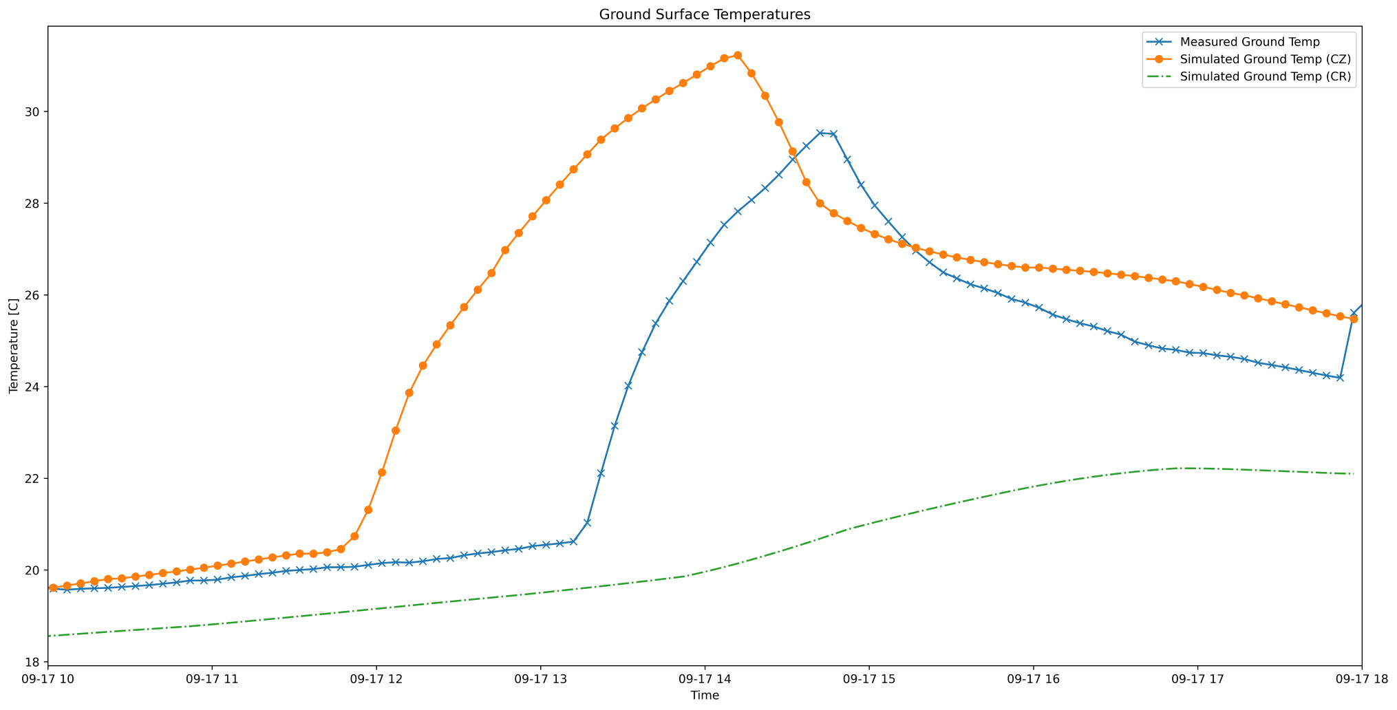
Model a shading canopy as a seperate thermal zone. I think the limit to this is that EnergyPlus wont consider the longwave exchange between thermal zones when they are separated by a large air gap (i.e Canopy and Ground, Canopy and surrounding buildings) (p41 of the engineering manual) .
Model the shade as the ‘roof’, the ground as the ‘floor’ and customise the walls so that they are as
non-existent as possible (i created open apertures at 95% of the wall face area, setting the properties of the window and face materials to as thin as possible, high conductivity and transmissivity).
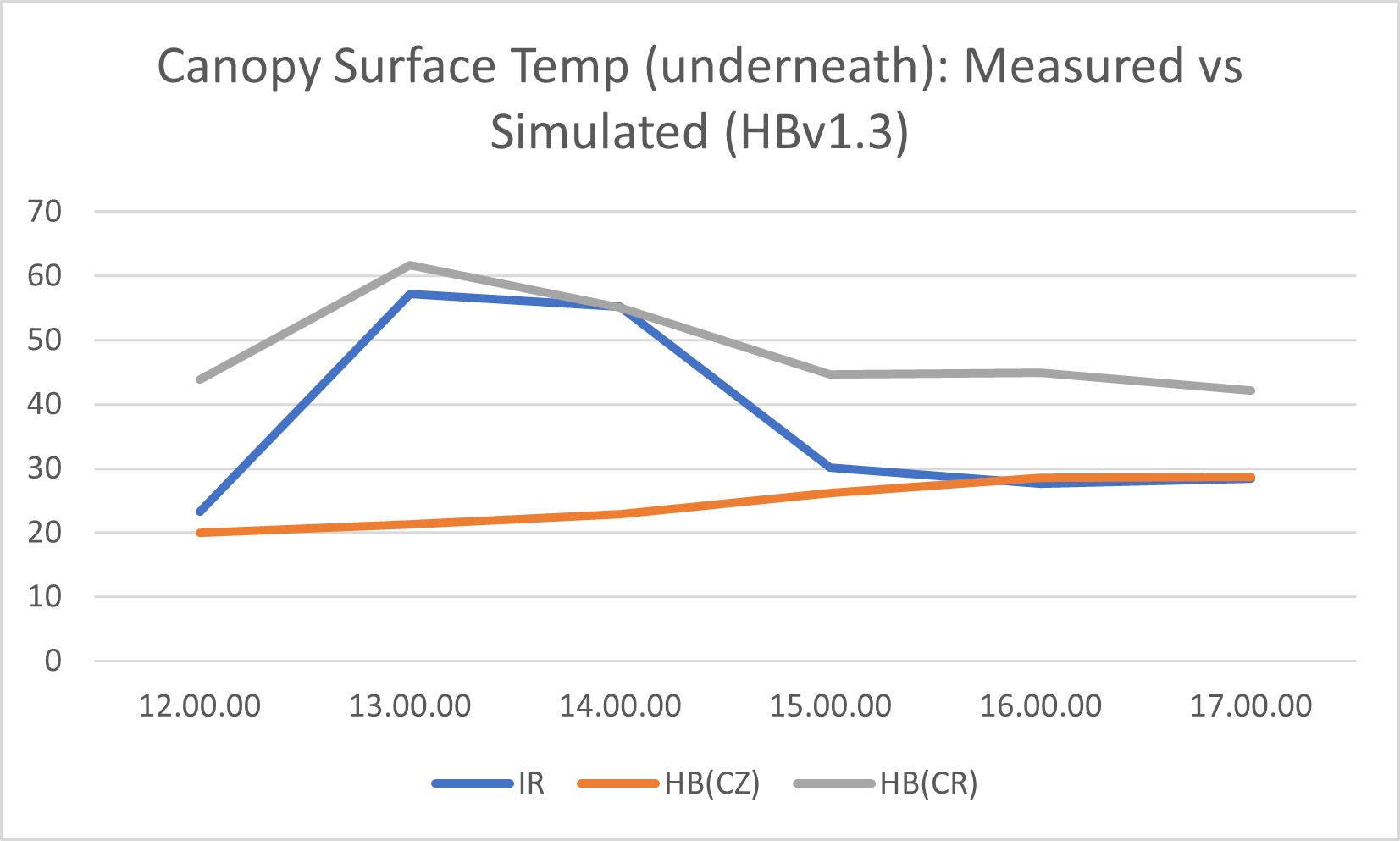
I have used exactly the same context, epw file, analysis period and simulation parameters but the first method limits how thin I can make the canopy geometry so I think that is affecting my results. This is what I’ve found.
It’s quite interesting …it seems like if I could combine the two methods I would have something that aligns with the measured temps (the blue line). Anyone done something like this before and would like to discuss method?
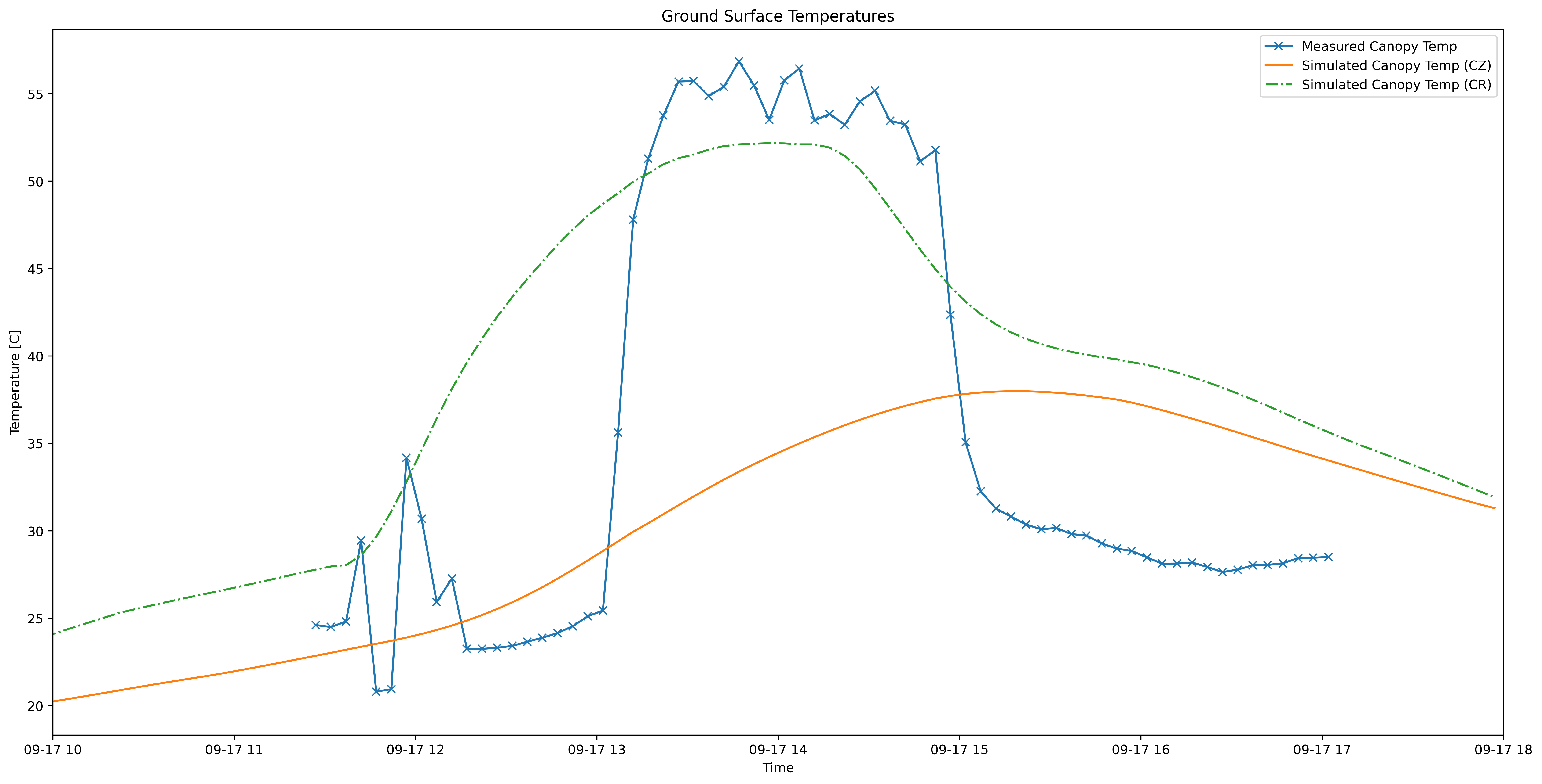
The CanopyRoom temperature seem much closer for both locations, but looks like its temperatures are more bufferered relative to the measured temperatures. This may be something you can refine by tuning material paramaters. This could be done by playing around with the emissivity, or increasing the thermal diffusivity of your materials \alpha = \frac{k}{\rho C_p} by reducing density, specific heat capacity, or increasing conductivity. Since the two surfaces are coupled, minor improvements could fix both.
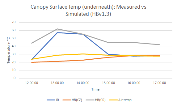
Can you also include the drybulb temperature for these plots? It’d be good to know what the difference is between the surroundings and the surface temperatures.
Hi @SaeranVasanthakumar
Thanks for the reply! I will have a go at playing with materials properties and see what I can come up with. I think that the ground materials properties definitely need adjustment as I’m using the default groundzone properties of ‘moist soil.’
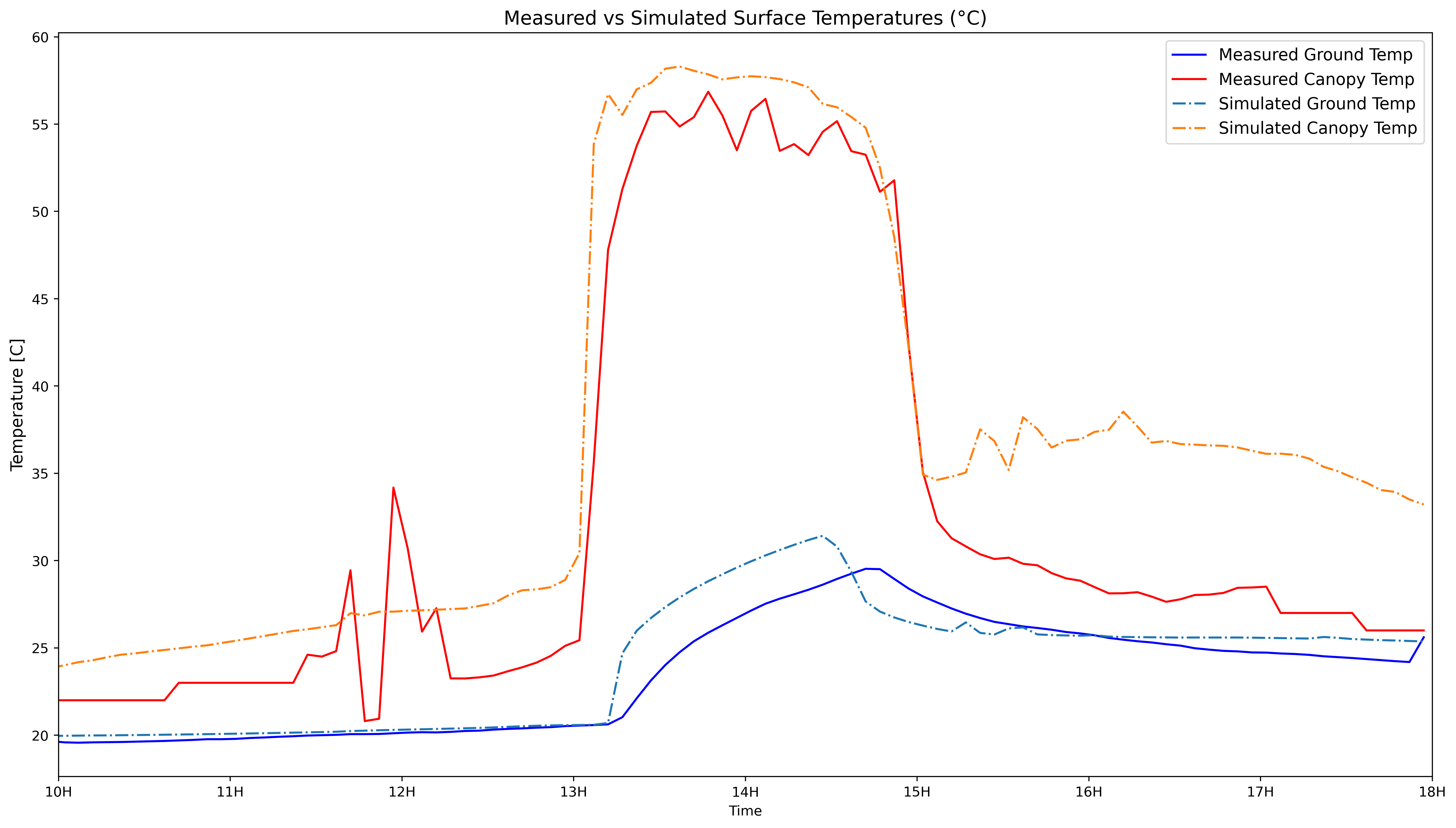
Here are the plots with air temperature included as well. I had some problems with the air temperature sensor in the morning so the values for the first hour are taken from the reported weather for the day (so not accurate to the exact location)
Thanks, it’s really helpful to see the air temperature. It definitly looks like the ground material needs to increase it’s thermal diffusivity, not only is it buffered, but you can also see the temperature lag relative to the surrounding air. Reducing the latent effect of ground moisture should definitly start to correct both those problems. So in addition to increasing conductivity, reducing density/specific heat capacity, you can also removing simulated moisture.
Also the ground seems cooler then it’s reference, while the canopy seems to be hotter then it’s reference, so I think increasing the reflectivity of the canopy and/or increasing absorption of the ground might help the surfaces get closer to their reference temperatures.
To answer your earlier question about whether this is a good way to model free-standing structures, I don’t know wha the state-of-the-art is, but I would say the CanopyRoom model could work (based on the evidence in your charts) as long as EnergyPlus’s radiation/reflection methods can be tuned to model the underlying solar radiation dynamics well enough.
I do wonder if there’s an alternative method where you can just use Radiance to better capture the solar radiation dynamics, and then solve for the difference in surface temperatures due soley to short-wave solar radiation by summing the direct, diffuse, reflected components, similar to the SolarCal method. I.e. solving for \Delta{MRT}_{sw} using: ERF = \epsilon f \sigma (MRT^4 - T_{srf}^4). Then total MRT is just the \Delta{MRT}_{sw} plus the MRT calculated from surface temps assumed to be equal to the outdoor air. Radiance won’t model the material heat balance, so this would only make sense if the reflected/direct/diffuse solar distribution on the ground and canopy has a much higher impact on the surface temperatures than it’s actual heat balance. Since the measured surface temperatures are very close to the the surrounding air at all times except for peak solar times, this seems like a reasonable assumption. In fact, if we assume the ground thermal mass is causing the bulk of your issues, one way of thinking of your problem is that the heat balance component of EnergyPlus is responsible for the bulk of your issues. But, as I said I’m not familiar with the state-of-the-art for exterior comfort models, so this is just speculation.
UPDATE:
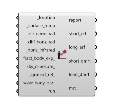
Turns out the Outdoor Solar MRT[1] component does what I’m talking about - using SolarCal to approximate surface temperatures (weighted by view factor to an individual). I was under the impression SolarCal was meant to be used for indoor spaces only, but I guess not.
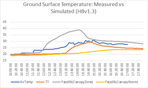
Hi @SaeranVasanthakumar, sorry for the delay in replying and thanks once again for your comments. I was playing around with the ground material properties as you suggested and ended up increasing the conductivity a lot (to 5 W/m-K) which brings the curve for the Canopy as Zone ground temperature relatively close to the simluation, although the peak temp occurs about 45 minutes earlier (see graph below). 5 W/m-K seems pretty unrealistic for soil but it does tell me that the simulation ground material needed to disperse more heat.
On the other hand, after adjusting material properties of the canopy (increased thermal absorbtion), I find the Canopy as Room surface temp curve more closely follows the measured data. (On a side note, adjusting the material properties of the canopy has no effect on the ground temperature)
On your points about calculating MRT - I did start looking at how different canopy materials could affect MRT but using the legacy Ladybug ‘MRT calculator’ and ‘Surface View Analysis Component’ to calculate longwave MRT (still requiring surface temps from EnergyPlus). I then plugged that into the new 'Solart MRT from Solar Components to account for shortwave radiation.
So far I found no significant difference on MRT when testing diffeent materials which seems to correspond to what you’ve said yourself. But I’m not sure how correct this part of my workflow so I need to look into it more.
You’re right that SolarCal was published in ASHRAE-55, which is an indoor comfort standard. But the shortwave effects of MRT over a human geometry are the same whether you’re inside or outside. The only real difference between the two is that you have a window between you and the sun on the indoors. So that’s why the “Outdoor Solar MRT” component still uses SolarCal under the hood.
In any event, it’s also my experience that shortwave solar and heat exchange with the sky has a much larger effect on MRT than the surface temperatures of the surrounding geometry. Assuming that these surface temperatures are close to the air temperature is usually good enough for a lot of thermal comfort applications.
Hi, I wanted to open this discussion up again because I’ve been working some more on modelling the canopy and made some definite improvements but also cant explain the reason for some of these improvements.
I went with the approach of modelling the canopy as the roof of a larger room (this: “1. Model the shade as the ‘roof’, the ground as the ‘floor’ and customise the walls so that they are as
non-existent as possible”).
Thanks mostly to the new V1.4 “Vegetation Material” component and the Opaque Material No mass component for the canopy, the simulated temperatures are reasonably close to the measured ones (see graph below) BUT only when I use the Polygon Clipping method for shadow calculation.
If i use pixel counting the ground temperatures follow a similar curve to what you see in the previous graphs. I guess this is because the pixle counting method is somehow not counting the windows as transparent (although the air temperature inside the canpoy room matches outside so some part of the EnergyPlus calculations are reading them as open). Can anyone explain why? Im submitting a conference paper on this pretty soon so if anyone can help me understand this it would be much appreciated!