Heat gain via window conduction in summer in a cool climate

This may be related to Understanding the Load Balance Component Assumptions.

We (@MichaelDonn and I) have another weird energy balance issue.

As you can see, in the cool climate of Auckland, New Zealand, we have a significant amount of heat gain via conduction through the windows for seven months of the year.

We cannot track the error in our logic and wonder if this is another case for @chris or a mistake on our part.

Any and all help gratefully received.

Anthony

SCRIPT REBUILD v7 HB ONLY TEST.gh (232.4 KB)
And here’s the test script - the result of the first week of Anthony learning the script as part of a summer scholarship research project…

It seems odd to me that, in addition to the heat conduction from outside to in, which would makes sense only in a much hotter climate, the Delta/Storage heat loss term in the graph almost exactly matches the Window Conduction Heat Gain…

Yet more list processing I do not understand.

The goal is to sketch model a small office building.

The test script converts a plane (Rhino Surface) drawn on a Layer named Plan. One then assigns a number of storeys and interfloor height, to generate a prototype.

Running some simple sliders for window areas and shading and wall depth and so on creates in put to an Ïdeal Loads" HVAC specification which then connects to a load balance.

With the HB Straight Skeleton we create 4 perimeter and 1 core zone for a ground a middle and a top floor.

Run straight through to the HB Annual Loads component produces this weird Load Balance:

We create the 3 levels by copying the base floor.

This creates 15 Rooms

In trying to figure out this we tried separating the list of 15 rooms produced by the Ideal Loads Component, and reattaching them as individual and then grouped inputs to the HB Annual Loads component.

Individually they worked as expected. In groups by orientation they worked as expected. Finally, we had them all attached, and they still worked as expected:

In other words, with this new list configuration connected to the HB Annual Loads component, the results were very different, with no weird Window Conduction Heat Gain!

The Delta/Storage component does seem worrisomely large.

But, I am thinking that I am missing something all important. Note: each level works well fed into the ideal loads. The error seems to be when we connect more than one level to the ideal loads component (with or without the inputs and outputs flattened)

Thank you in anticipation of your kind responses

I have identified the source of the problem, but not the solution!

The issue is the circled component in this image.

The idea of a multiplier is that when we model a multi-storey tower, we model the top and bottom floor, then the representative intermediate floor is multiplied by the number of intermediate floors there are in the tower.

It is the inclusion of this multiplier that is creating the problem in the output.

WITHOUT the multiplier but combining the three levels

WITH the multiplier and combining the three levels

WITH the multiplier, but just the middle level

WITH the multiplier and the ground floor plus the (multiplied) middle floor

WITH the multiplier and linking all three outputs to the next hb_objs input in the chain

Why adding more levels to the inputs should now make the energy flows per square metre any bigger is beyond me. And why the previously used grasshopper component should do something different is also WAAY beyond me?

==================================================================
In Summary:
with the levels combined via a component where

  • Input D1 is the ground Floor,
  • Input D2 is the (multiplied) middle Floor(s)
  • Input D3 is the top Floor
    The result is this weird Window Conduction is Heat Gain not, as the climate would imply Heat Loss

But,
with the levels combined via a component where

  • Input D1 is the (multiplied) middle Floor(s),
  • Input D2 is the ground Floor
  • Input D3 is the top Floor

The result is

AND WITHOUT the Multiplier and with the three levels via a component where

  • Input D1 is the ground Floor,
  • Input D2 is the (multiplied) middle Floor(s)
  • Input D3 is the top Floor

The result is this:


Given that the middle floor is multiplied this last graph is what the results should look like, even when the multiplier is applied as the results are per square metre!

Hi @MichaelDonn ,
Don’t have a solution for your questions, but have some comments.
Is there something in the workflow when using multipliers that is not clear (to me) in the HB interface and i believe is what is making you trouble.
If i wanted to use the multipliers in your case i would use only one floor and give, say, 9 as a value to multiply. This will include the ground, middle and top floors. This is how the option works in Dragonfly (i believe).
In your case you are moving the middle floor to be somewhere at mid height. The multiplier will take this floor and “copy” it from that place above it. This is a mistake (almost) for sure. BTW, the calculation of this height is wrong. It is 17.5 and should be 20.
Question: when you use the WOTHOUT multiplier option, do you solve the adjacencies between floors? Didn’t see that in the GH file, where you solve that at the floor level.

I’ll be glad to understand how the workflow with multipliers should be in HB.
Also i wish to have the possibility of visualizing the building fully (with the multiplied floors) as DF does.

Until all this is clear i recommend to model the whole building. @chris 's comments are needed here to shed some light.

A.

Thanks @AbrahamYezioro - you make some interesting points that challenge my understanding of how LBT works.

in my mind, there is a huge difference between modelling for appearance (for the model to look like the final building) and modelling for accurate and efficient representation of energy performance. The way we are modelling has been the convention for accurate energy modelling for decades.

This approach was confirmed by a paper out of NREL https://citeseerx.ist.psu.edu/document?repid=rep1&type=pdf&doi=744a45dbc6b04a9f399a2f55b4d9edcbf3fd2b2d

Back in 2005 in relation to the original plans for the super-tall Freedom Tower Ellis and Torcellini concluded that multipliers give an accurate picture of even that 100 floor building “…as long is that [multiplier] floor was at mid-height.” They did note that if that building was in amongst a bunch of other lower buildings, then the shading from them might need a multiplied floor mid-height amongst the nearby shading buildings, plus another with a different multiplier for the floors above the shading buildings. The majorly different floors, the ground and top floors, need to be added to these multiplied floors because the ceiling and floor of the multiplied floors are not modelled as adjacent to the other floors, but as being adiabatic.

Li Jing, in a recent PhD looked more closely at the effect of the adjacent buildings Urban Microclimate Analysis for High Performance Office Buildings. This combined CFD modelling (Butterfly of course) for local winds, UHI modelling, incorporation of the decrease of temperature with height and demonstrated clearly that these microclimate effects can make a 20+% difference in the energy use.

To my knowledge, the approach @anthony.schneider is taking is energy modelling good practice. The multiplier in EnergyPlus practice just takes the mid floor (at the half way height point) and multiplied the results for those rooms/zones by the multiplication factor. No increment in building height.

M
.

Hi @MichaelDonn ,
Interest discussion becouse it will set, hopefully, the correct workflow in LBT.
Though i’m not using multipliers frequently i’m aware of the advantages in doing so, especially on high (rise) buildings. Thanks for the sources.
Made some homework after your last post. You are right the recommended way of modeling the mid floor is locating it at mid height. You can see that here in bigladder. They recommend for very high buildings to model more than one mid floor.
Saying so, i also checked the workflow used in the DF example rooms_to_stories_to_building. There the approach for the multiplied floors is not as the previous comment. The copies start from the modeled story and above.
Attached one version of the file, where I isolated the mid floor in the example.
rooms_to_stories_to_building_AY.gh (246.7 KB)

Right now i’m a bit of confused about what the “correct” procedure would it be in LBT. Hoping @chris make this clear.

-A.

Hi @MichaelDonn,

I took a look at your script and think the problem come from assigning “Air boundary” to the adjacent geometries.
I had some similar issues with Airbounadry balance visulization. I think since in airboundary enegy plus models them as solar enclosure HB balance might be still have some troubles to assign them on proper rooms as stated in this post

When I dissable the airboundary the results becomes as expected:

1 Like

Thank you for demonstrating this @Hamidreza.

Air boundaries between zones on a particular floor allows heat and radiation flow, but not mass (air) transfer. This should be a standard, default approach allowing daylight for example to spread across the core as well as perimeter zones.

However, I will look into testing this idea further. We certainly want to model a building that is open plan, not one with separate “rooms”, even though the terminology of LBT is about “rooms”.

1 Like

Thanks for the discussion here, @MichaelDonn , @anthony.schneider , @AbrahamYezioro and @HamidrezaSh ,

This has all made me take a closer look at the load balance and I have made a three tweaks that should generally help things become more balanced. They are all in the PR I just merged here:

I will start with the tweak I made that is the most relevant for this particular model:

  1. Missing Back-Reflected Solar - After studying this particular case in detail, I realized that the main reason why the storage term is so high is not because of the room multipliers or even the air boundaries but rather the fact that the model is very glassy with a load balance that is dominated by solar. Given the way that we had been constructing the load balance, the solar term accounted for all of the transmitted solar and the conduction term accounted for all conduction through the window (including the impact of both outdoor temperatures and solar that gets absorbed by the glass and then conducts to the interior). However, I was not accounting for another important part of the solar calculation - the shortwave solar that gets transmitted through the window but then reflects off the floor and then back out of the window. We have been missing this for all models to date but it really only becomes noticeable when you have balances like this one that are dominated by solar. Most of the storage term that you are seeing in this case is back reflected solar. I spent a few hours looking through the RDD files and the EnergyPlus Input/Output Reference for the output that would tell me this back-reflected solar but I could not find it. It seems like there used to be this Surface Window Shortwave from Zone Back Out Window Heat Transfer Rate [W] output but it’s clear that these docs are out of date and this output has been changed or removed from the current version of E+ we’re all using. But the rest of the docs on the window outputs make it very clear that there is solar being reflected back out the window. I plan to open an issue on the E+ Github but, for now, I just ran some tests and found that this back-reflected solar seems to pretty consistently be ~6% of the total transmitted solar. So, to address this for now, the change I made above is just multiplying the transmitted solar term by 0.94. This should practically eliminate the storage term that’s in @HamidrezaSh 's screenshot.
  2. Service Hot Water was not Respecting Multipliers - I did some extensive tests with multipliers just to be sure that this was not the issue but the only thing that I found was that the service hot water was not respecting the multipliers. Usually, we don’t notice this since SHW makes up such a small portion of the balance but it might have been adding up on a larger building like this and causing us to blame that instead of the other factors. In any event, this is fixed by the tweak above
  3. AirBoundaries Should Use a High Timestep - I was able to create a lot of the the issues that you note about AirBoundaries, @HamidrezaSh , and they were occurring primarily because this is not true of Honeybee AirBoundaries, @MichaelDonn :

Air boundaries allow you to keep the room air nodes separate from one another but you get both radiant heat transfer as well as zone air mixing across Honeybee AirBoundaries. This more accurately represents a case where the boundary between rooms does not represent a real surface in reality.

To get back to the reason why you should use a high timestep with AirBoundaries - coarse timesteps like 1 per hour cause some imbalances between this air mixing between Rooms and the hot/cold air delivered by the HVAC system. Increasing the timestep to something like 6 (or 12 for good measure) usually gets this type of imbalance to go away. FYI, this is also true of window-based natural ventilation (as I think you are aware). I just added a new warning to the HB Annual Loads component, which will alert you to cases where your timestep is low and you have air boundaries in the model:

Once you increase the timestep, the warning will go away and the loads will become more balanced:

3 Likes

Great to see the refinement and development of the tools based on these studies.

I am a little concerned about applying a factor to correct the solar element, I know @milo.g and @rahulgrover18 have done a fair bit of analysis trying to align IES and HB results when it comes to solar, I think they reached their own conclusions but I was never fully satisfied that we had cracked it and it’s something on my long list of things to come back to.

I suspected solar reflected back out of windows could be part of the discrepancies we found.

It’s interesting that the output may have been stripped from E+, and trying to find details of IES backend calcs is always a challenge.

In reality, when buildings aren’t typically empty boxes with uniform surface properties I do wonder how much solar will actually make its way back out of a building.

Food for thought!
Cheers,
Charlie

I’m 100% there with you @charlie.brooker . The correction factor was really meant to be temporary until I could figure out what exactly is going on.

I have managed to create a dead simple example that illustrates the problem and I have asked the EnergyPlus developers here. It’s very clear to me that we’re missing something when we use the E+ outputs we’re currently using to construct the load balance and it’s all related to solar and envelope heat transfer. Hopefully, the developers can clear this up for us and tell us where this ~6-7% of solar energy is going if it’s not leaving through the building envelope.

I also have a correction to make in that E+ didn’t strip out the output. I was just dumb and didn’t realize that I need to use Output:Diagnostics, DisplayAdvancedReportVariables; in the IDF if I want to be able to see that E+ output. Michael Witte made this clear for me here. That said, I have looked at that E+ output and it didn’t match up with the missing solar energy so it seems that actually was not the issue. Hopefully, the E+ developers can say exactly what’s going on.

1 Like

Thanks a lot, @chris for your thorough reply. I learned much from your response.

I have a question when I tried to rerun @MichaelDonn’s script with the new release and increased time steps I am still getting similar results that show heat gain from window conduction in summer months.

I checked and made sure that the HB core had been updated and restarted Rhino several times to be sure. Am I doing something wrong here?

When I run the balance separately for each floor and then combine the results manually the graph results look as expected. Don’t know though it is the correct approach!

When I do the same for the variant without air boundaries the results of both approach look the same

Thank you @HamidrezaSh

And, we come back to my concern: heat conducted IN from outside when we use the multiplication option, which is the recommended approach for tall buildings, we get results that we do not trust. It is NEVER that hot outside that the heat conduction from outside would be of a similar size to the heat gain from solar radiation. If I start with the https://solarview.niwa.co.nz/ web site I can estimate that a North facing window of 1 square metre would gather at its highest ~400W on average over an hour.

Over the year NIWA report in Wellington the following monthly solar gains / sq m

Cumulative kWh/m2
Jan 2.48
Feb 2.85
Mar 2.88
Apr 2.64
May 2.09
Jun 1.76
Jul 2.03
Aug 2.5
Sep 2.64
Oct 2.57
Nov 2.4
Dec 2.33

The fact that the data in the Heat Balance is per square metre of floor area requires us to do a little more arithmetic.

if I have a square metre of double glazing (rough R-value 0.25 m2 degC/W) then I have a U-value of 4 W/m2 degC. To obtain a heat gain approximately equal to the absolute maximum of 400 W/m2 with this U value would require a temperature difference of 100 degC between outside and in. This would mean for a normal interior temperature goal a temperature outside of 20degC above the boiling point of water. I suspect I have something wrong in the logic of this calculation, but cannot figure it out at present.

I suspect a simple coding error arising from the multiplier as it is coded, but can go no further in the analysis at present?

1 Like

Thank you for the analysis @chris. As thorough as always.

I am surprised that the highly solar driven situation has not arisen in the past - with all the rhetoric against highly (over?) glazed office buildings, I had assumed that 70% WWR would have been common.

I feel I should be apologising for this added workload, but am keen to ensure that this fabulous tool is as informative and reliable as possible. It is useful from 1st year introduction classes (revolutionising how one discusses Passive Solar Design) through to PhD study and - it turns out - to Design Leaders in large architecture practises. With a cheat sheet explaining how to read the various components it is such a hugely informative design tool. (I retain my concern at the “storage” label - and feel that the “Mechanical Ventilation” term also requires more carefully explanation/labelling).

In this case it has reported something that I believe demonstrates its utility in Quality Assurance. It is clearly showing something that does not, and should not, feel right (window Conduction as a huge positive term)

1 Like

Hi @HamidrezaSh,

Thank you for investigating the window heat conduction during summer after the new release, and how the multiplier node might be creating these strange results.

Could you please attach your modified Grasshopper file so that I can take a look - I’m unsure how you multiply the modelled middle floor by the actual number of middle floors based off your screenshots alone.

Please let me know how you go about multiplying the middle floors.

Kind regards,
Anthony

1 Like

Hi @anthony.schneider
Sure, here is the file
SCRIPT REBUILD v7 HB ONLY TEST (1).gh (260.0 KB)

Hi @HamidrezaSh,

Thank you for providing the file - this helped a lot in understanding your edits to the script and how you produced these results.

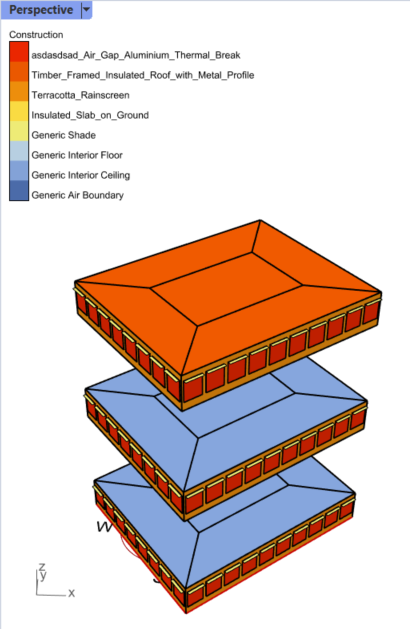
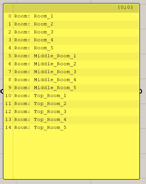
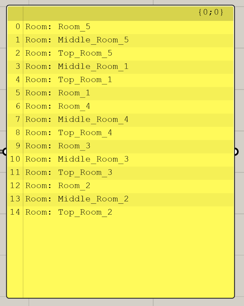
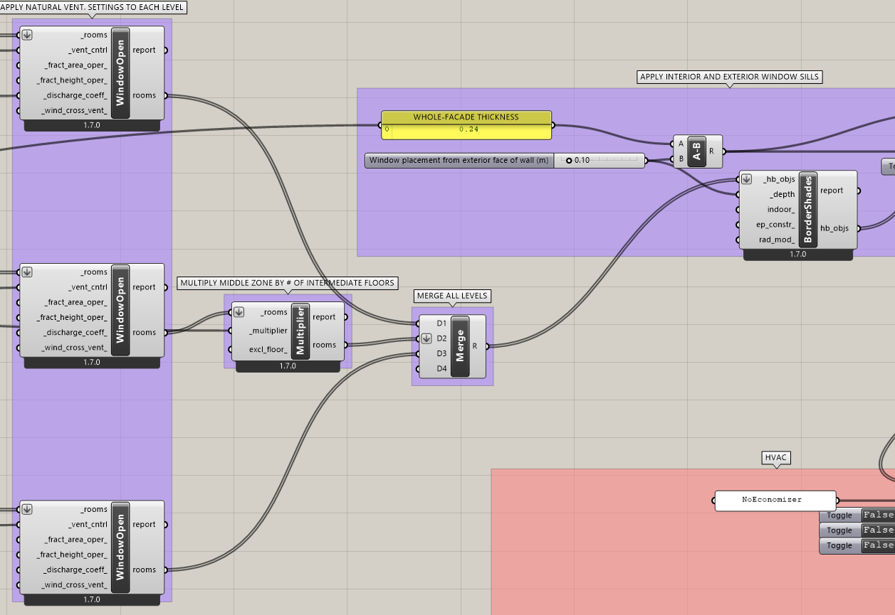
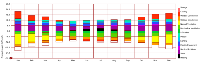
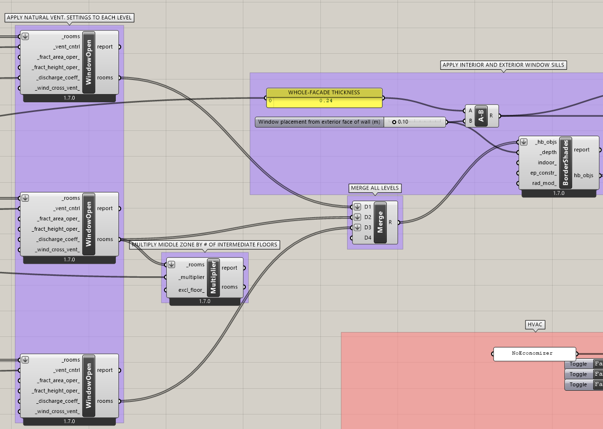
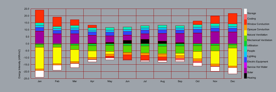
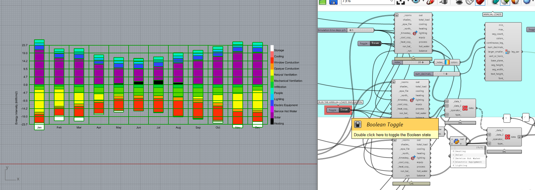
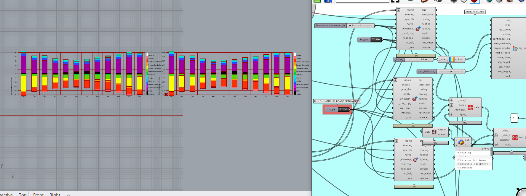
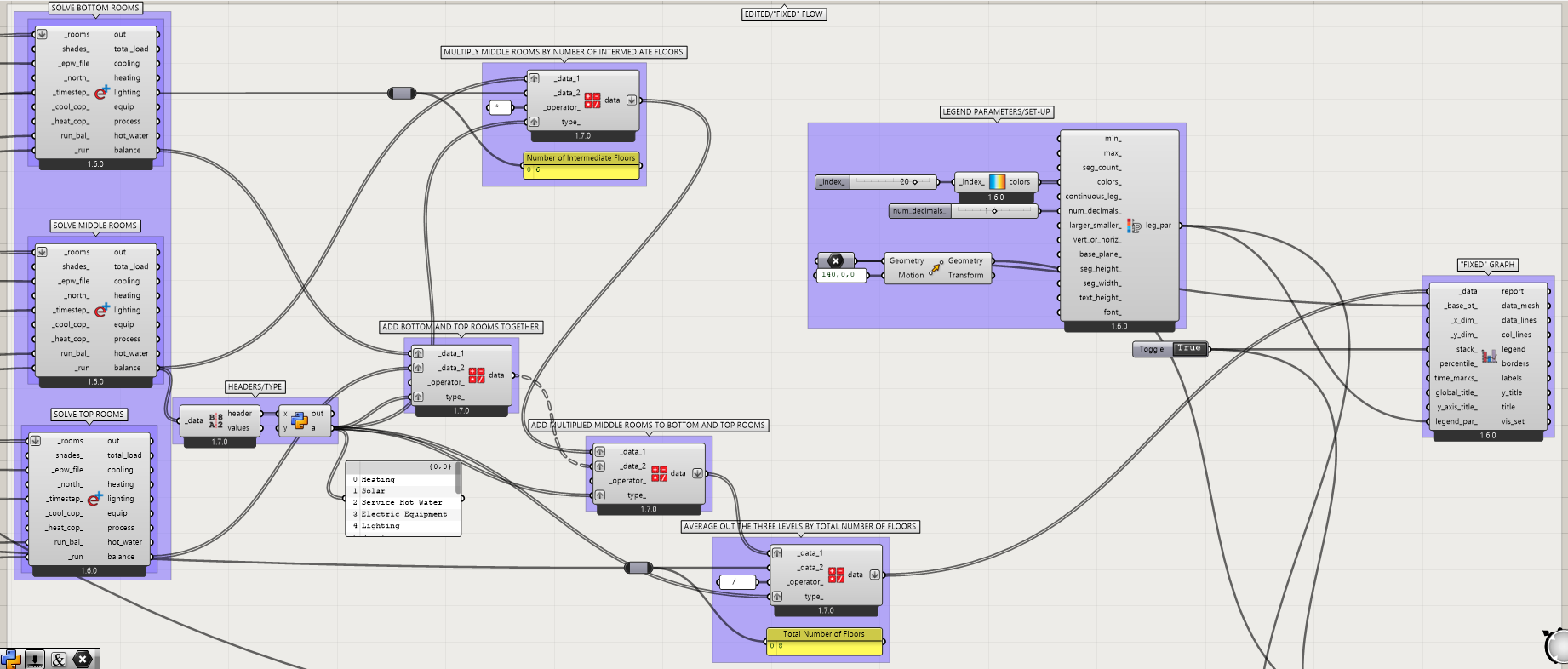
Am I correct in saying that your script doesn’t multiply the middle floor, but instead separates the three levels (using 3 chunks of 5), solves them separately, adds the data of each floor together, and then averages the data out by dividing the results by 3 (for 3 levels)?

However, to recreate the multiplier for the multiple middle floors, the data for the middle floors could be multiplied by the number of intermediate floors, and then added to the bottom and top floors, and then the summed data being divided by the total number of floors.

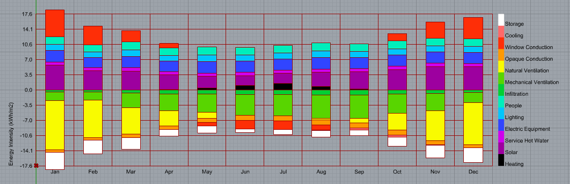
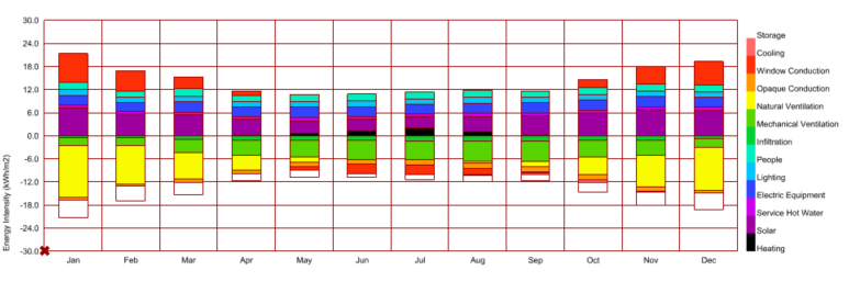
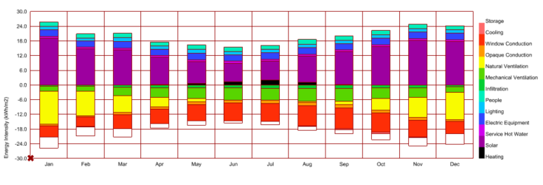
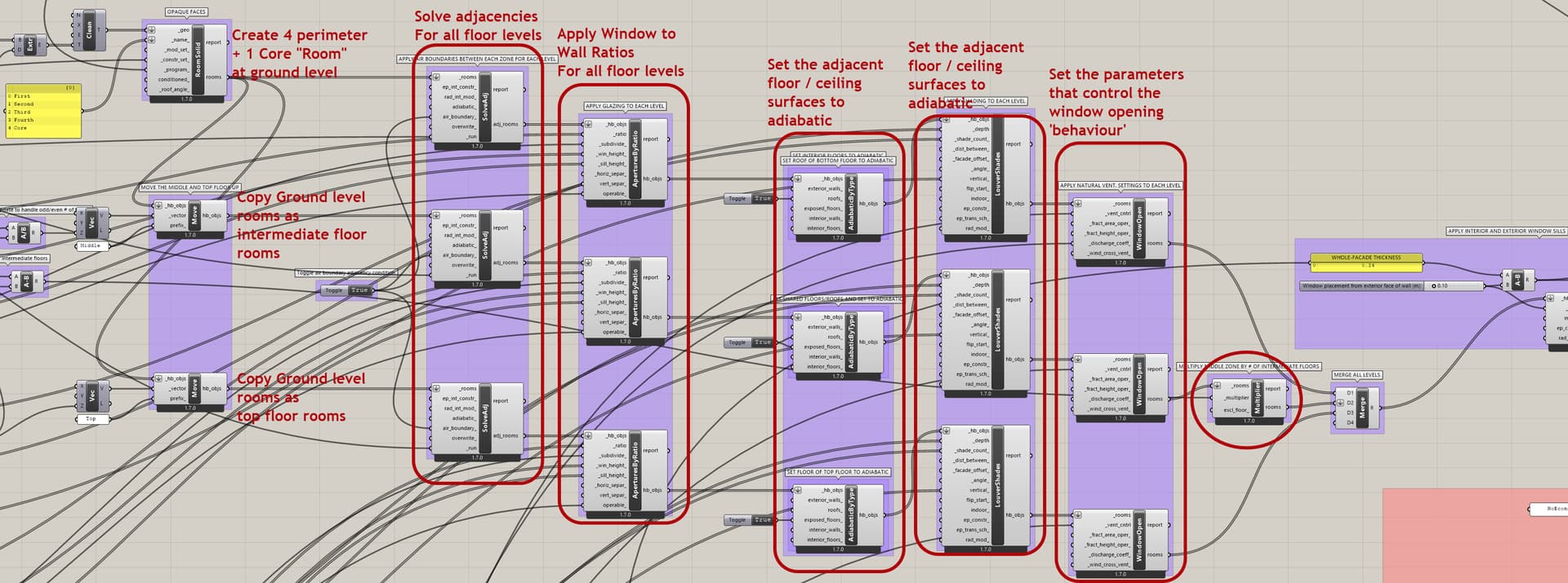
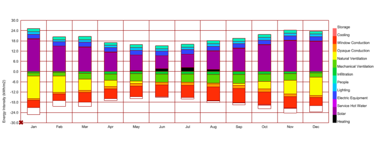
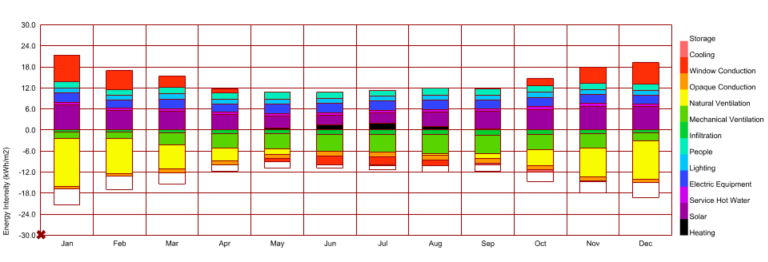
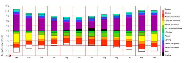
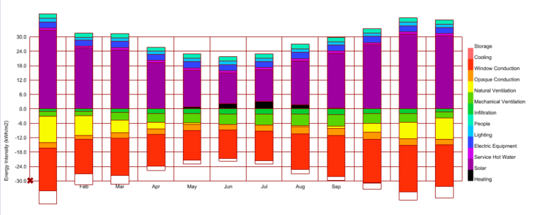
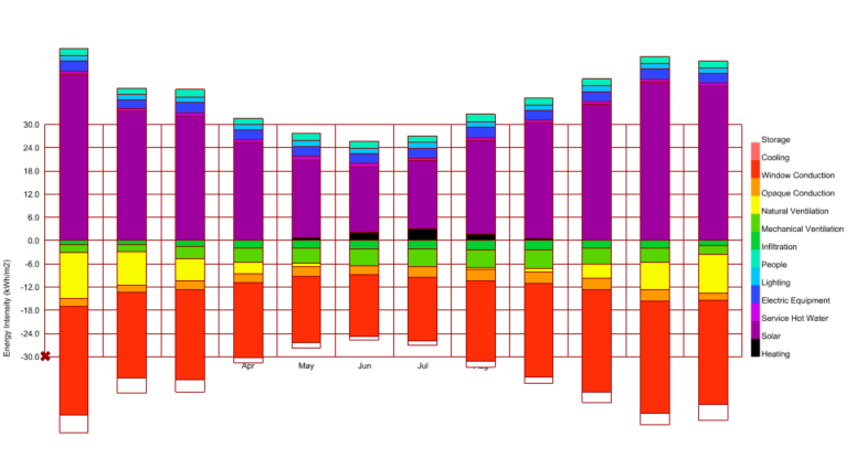
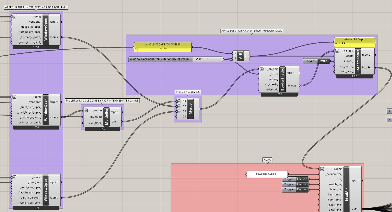
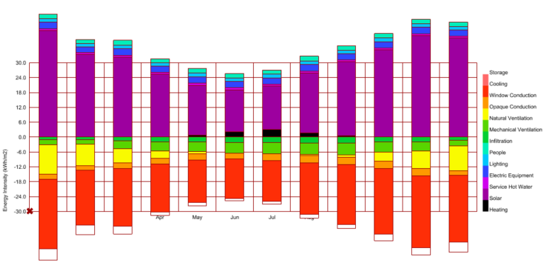
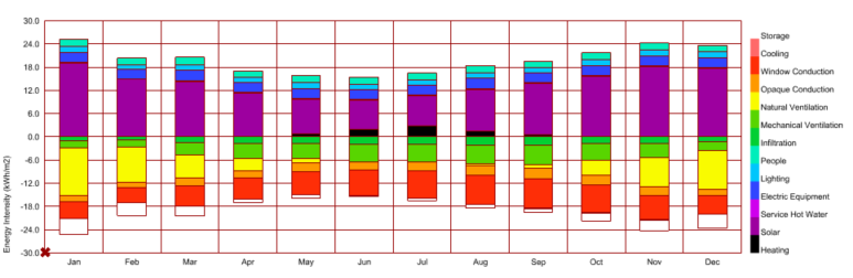
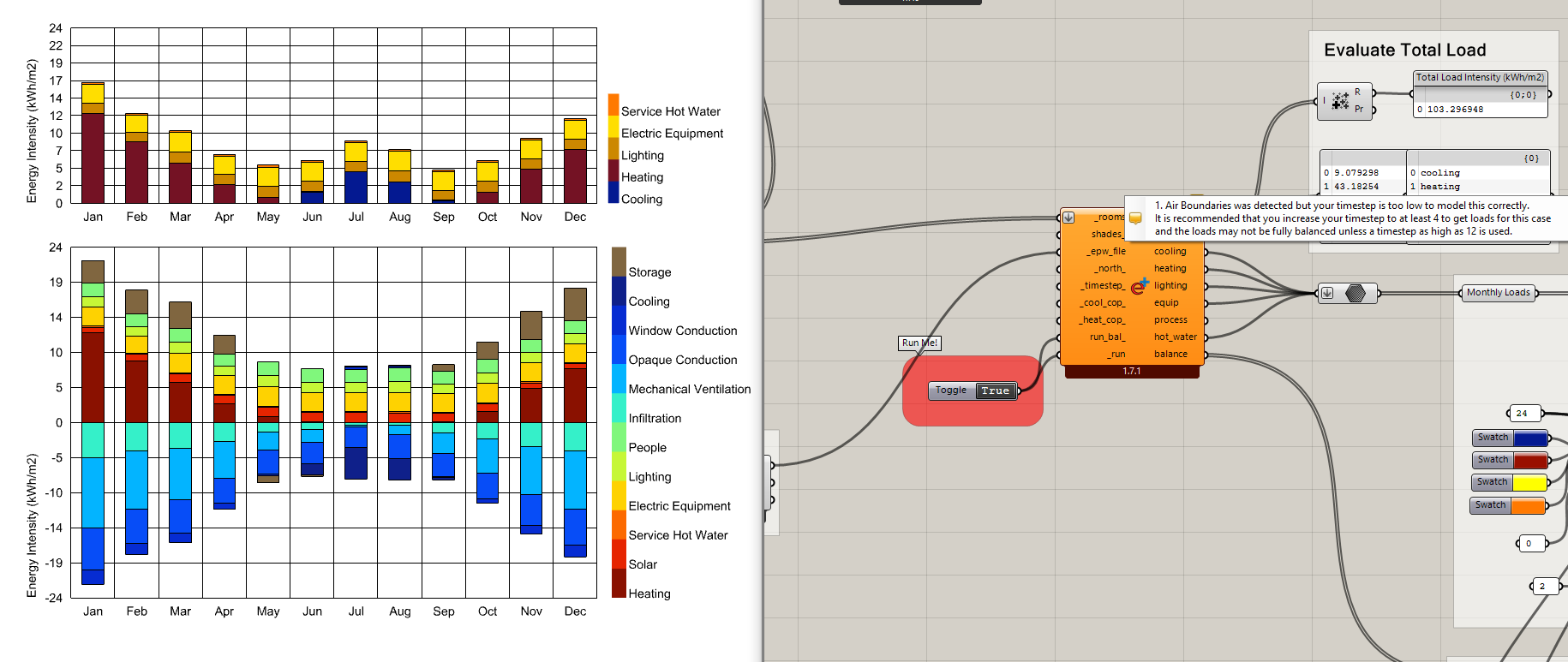
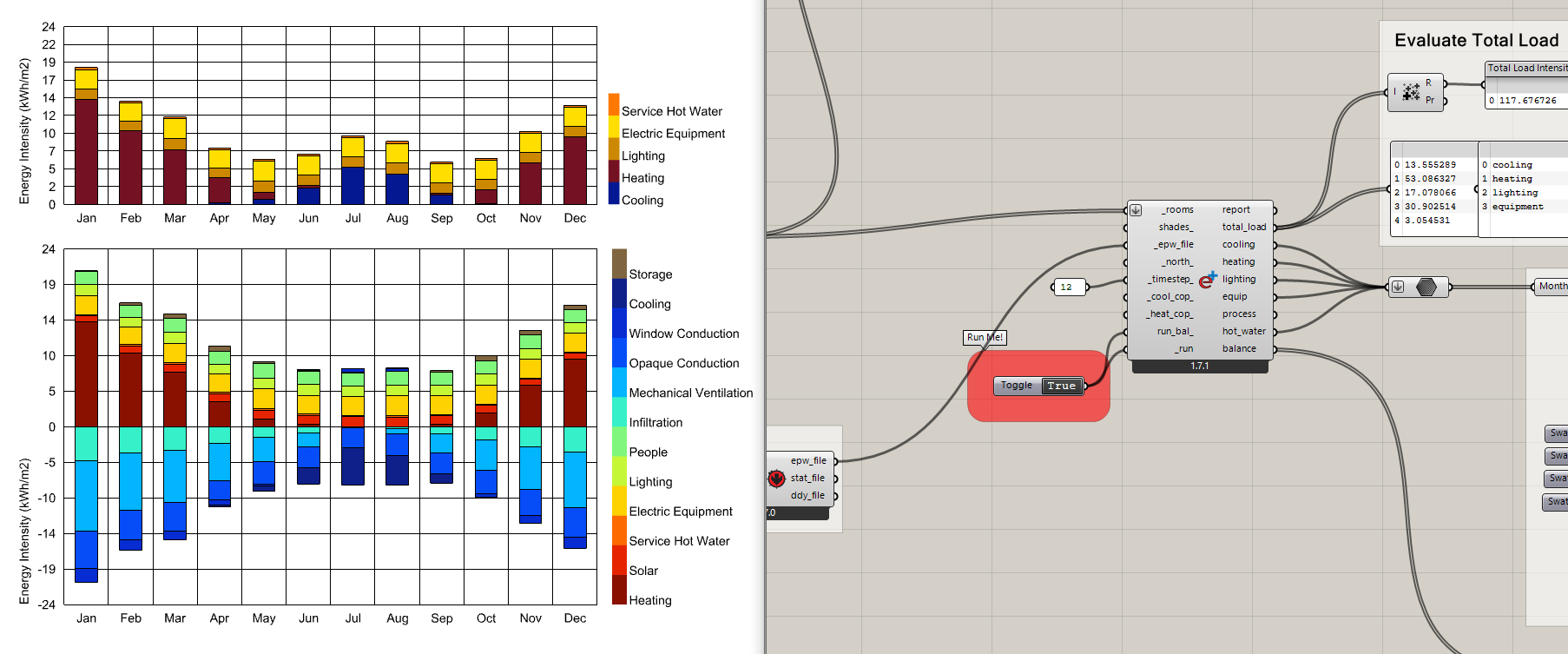
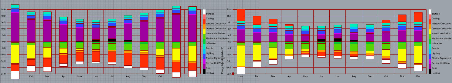
I have made these changes to your script (see first image below), and the results still look believable, with no summer heat gain from window conduction. The results of the edited “multiplier” script are on the left, and the results of the solver logic from my original, un-edited script are on the right (see second image below).

(Air boundary is set to true in my investigation)

Regarding your question about not knowing if this is the correct approach, this method does avoid the potential list processing issue and produces believable results - but will each full simulation take longer due to needing to run 3 separate solvers?

I tested the time to solve on my machine, in a not-so-scientific manner and the results were:

Using the original script (produces weird results): 112.8 seconds
Simply reordering the list from the original script (produces believable results): 123.7 seconds
My slight modifications to @HamidrezaSh’s experiment (produces believable results): 93.7 seconds.

So perhaps your method is the right way to go about this problem @HamidrezaSh, since it ran the fastest and gives reliable results… this will be important when running a parametric study.

Looking forward to potentially seeing how yourself and others in this thread interpret these results and thoughts!

Kind regards,
Anthony

3 Likes

Quick check @anthony.schneider .

Have you implemented the fix that @chris has published has been implemented in your version of LBT? Linked here again: fix(loadbalance): Tweak a few of the load balance terms by chriswmackey · Pull Request #987 · ladybug-tools/honeybee-energy · GitHub although it is waay up this chain …

1 Like

I have no contribution to make to the conversation but I just wanted to say that reading through this conversation made me happy! It has been a while since I have read such an in-depth conversation on the Ladybug Tools forum. Not that they are not happening. I just haven’t had the time to check them. The community of experts working together at its best. Cheers everyone! :raised_hands:

5 Likes