Great Ladybug Tools Community,
It’s that time again when we are happy to announce another release of the Ladybug Tools (LBT) for Grasshopper (version 1.4.0)!
You can download it from Food4Rhino and install by following the instructions here.
For people who already have an older LBT plugin installed, the Food4Rhino download for version 1.4.0 includes an uninstaller.gh file that can be used to completely uninstall your old version before installing the new version. While uninstalling isn’t a requirement, it is recommended to ensure everything about your installation is up-to-date. And don’t forget to update to the latest compatible version of OpenStuido and Radiance listed in the compatibility matrix.
Since the last release, we’ve fixed a substantial number of issues and bugs thanks mostly to the members of this community running larger simulations than ever before, delving deeper into the results, and running the software in a variety of configurations. A big thanks is owed to anyone who reported issues. Because of your efforts, version 1.4 is now more reliable and robust than ever before!
Now onto the exciting part of all the new features included in version 1.4.
Ladybug Features
Bake Colored Meshes to Hatches
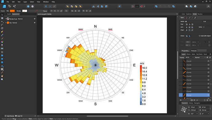
Back by popular demand from the Legacy plugin, there is now a component in LBT 1.4 to bake the colored meshes that form the basis of most of the ladybug graphics into Rhino hatches. This is particularly useful for those wishing to export ladybug graphics to other vector-based programs like Adobe Illustrator, Affinity Designer, or Inkscape.
Click to read more
In all cases, the Rhino hatches will be imported as colored vector polygons to these platforms. The hatches are also useful for exporting vector-based PDFs directly from Rhino for those cases where your architectural drawing set could benefit from your ladybug graphics.
Set the Rhino Sun
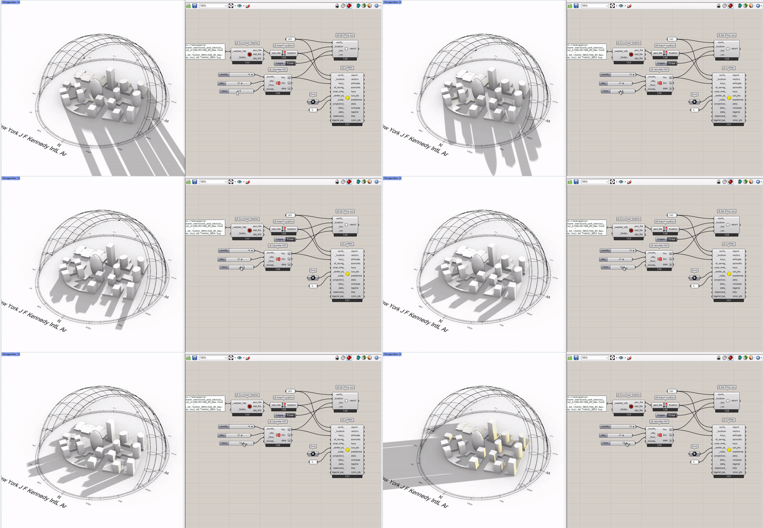
Another Legacy component making a comeback is the “Set Rhino Sun.” The component is particularly useful in cases where you don’t need the precision of a direct sun study and you just want a quick general picture of where shadows are as you scroll through the hours of the sun path.
Writing Data Collections To/From CSV
After it became clear that many workflows could benefit from the ability to write data collections to files and load them back in other scripts, we’re happy to say that LBT 1.4 includes Dump Data and Load Data components exactly for this purpose. By default, all of the data collections that you plug in to the component are written into a single CSV file, which is not only a smaller file size than most other options but is also more human-readable and import-able to spreadsheet programs for analysis outside Grasshopper.
Click to read more
Options are also available to export data collections to JSON or compressed PKL files. All 3 formats can be read by the “Load Data” component so that data collections can be loaded back into Grasshopper exactly as you had them.
Monthly Chart Display Improvements
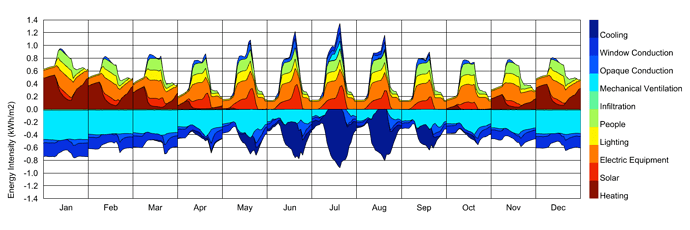
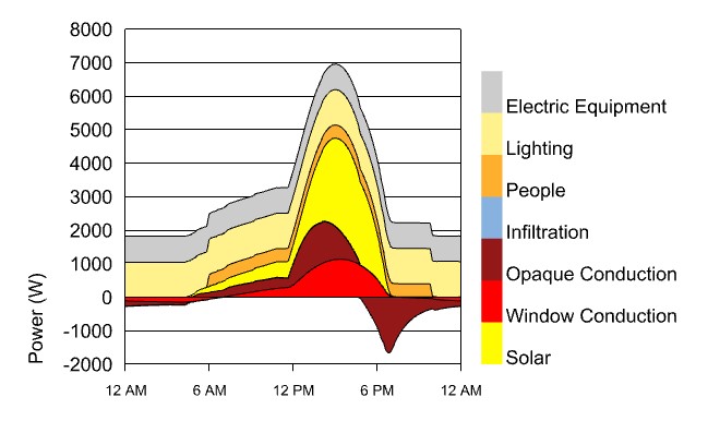
While we usually wouldn’t devote a whole release note for an incremental improvement of an existing component, this one was cool enough that we felt the need to have one. The methods under the hood of the Monthly Chart have been improved such that data now stacks on both the positive and negative axes of the chart. This allows for the construction of graphics like hourly energy balances, where terms that can change from positive to negative with the seasons will display on the correct side of the chart.
Click to read more
We’ve also added an option for time_marks_, which can be used to display the hours of the day on the X axis of the chart. It’s particularly helpful in cases where the chart is displaying a single day of data, as you would for a peak load study.
Radiance Features
Better Parallelization Without the Need for Sensor Count
In LBT 1.4, we continued to improve the parallelization of all Radiance simulations by implementing methods to evenly distribute the sensors between the available processors. This replaces the older parallelization method that relied on people specifying a _sensor_count_ for how to subdivide the model grids. While the performance improvement of this change is different depending on the type of model, we found that these new parallelization methods reduced simulation time by about ~25% for typical models containing a few rooms. Perhaps more importantly, modelers no longer have to question whether they supplied the best _sensor_count_ for their simulations since we can now all rest assured that the best subdivision of sensors is happening under the hood.
Extract HDR Component
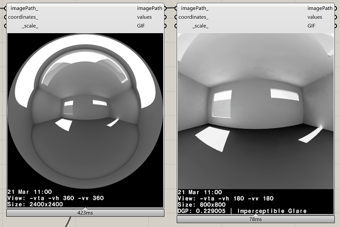
Thanks to the efforts of @mikkel, the LBT 1.4 release includes a nifty component that can extract individual HDR views from spherical angular fisheye Radiance renderings.
Click to read more
The component is particularly helpful in cases where you want to process multiple view directions. For example, you know that an occupant will be seated at a given location in a room but you want to study the glare this occupant would experience as they look around the room. Now, you can run a single view-based simulation of one 360 degree rendering and convert this result to several different 180-degree HDRs for glare analysis without the need to re-run the whole simulation for each direction.
More information on the component can be found here.
Energy Features*
*Most of the energy features listed below apply to both the Dragonfly workflows and the HB-Energy workflows.
Process Loads
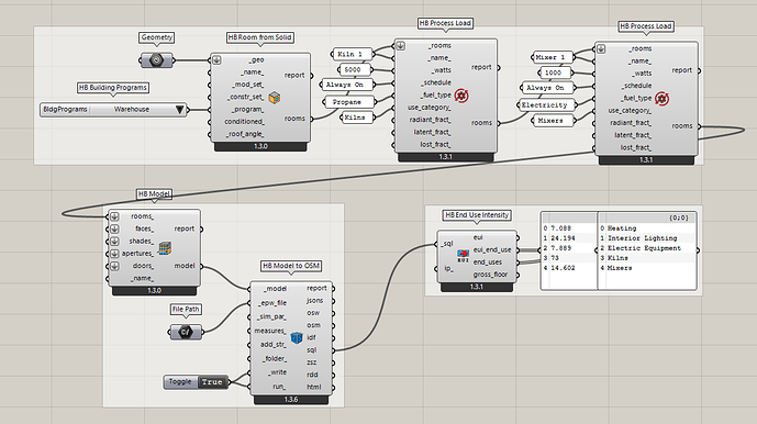
If you’ve modeled enough buildings, you’ve probably encountered equipment that doesn’t fit neatly into the “electric” or “gas” per-floor-area categories used by Honeybee. Whether it’s a wood burning fireplace, an industrial autoclave, or a piece of manufacturing equipment, certain processes can present challenges about how to model them. It is for this reason that we’ve added a dedicated Process Load component in LBT 1.4.
Click to read more
The component allows maximal freedom in terms of the fuel type and fractions of heat that are lost/latent/radiant. You can also use them in series to add several different process loads to the same room and get each item reported separately in the end uses. Process loads can also be used to represent certain specialized pieces of equipment to be separated from the other end uses, such as MRI machines, theatrical lighting, elevators, etc.
Detailed Service Hot Water (SHW) Systems
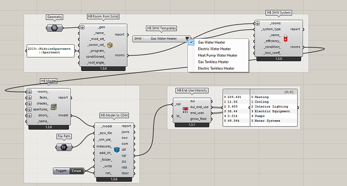
While the last two stable releases allowed you to simulate heating demand for service hot water, it was not possible to model the equipment supplying this heat or get the electricity or fuel it consumes. That has changed with the 1.4 release, which has introduced several detailed SHW system templates that can be applied to rooms to meet their hot water load. Both traditional fuel-burning systems and newer heat pump and on-demand systems are available, allowing you to compare the energy savings of different heating technologies.
Click to read more
The SHW templates were modeled after how the HVAC templates work in that, as long as they are assigned to a Room with a hot water load, they will be used to meet that load. Just like how HVAC templates assigned to rooms with setpoints will meet those setpoints. If no SHW system has been assigned, just the raw SHW heating demand will be reported in the results. The detailed hot water systems include a few straightforward properties that can be used to customize them, such as heater efficiency/COP and the ambient conditions in which they operate.
More Face Attributes to Visualize
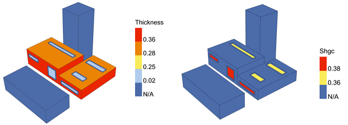
In addition to the R-Values and U-Values that could be visualized previously, you can now visualize the construction Thickness [m], Density [kg/m2], Heat Capacity [kg/K-m2], Solar Reflectance, Solar Transmittance, and (perhaps most importantly) Solar Heat Gain Coefficient (SHGC). The last attribute is computed using a steady state heat balance method similar to LBNL WINDOW but the properties better reflect how EnergyPlus interprets the window material properties.
Annual/Peak Loads of Detailed HVAC
Thanks to some recent improvements, each of the detailed HVAC templates can now be translated to an equivalent Ideal Air System. This means that essentially any Honeybee Room can now be used with the Annual Loads and Peak Loads component, regardless of the assigned system.
Click to read more
Properties like heat recovery and demand controlled ventilation are translated from the detailed to the Ideal Air system and detailed templates that only perform heating or cooling have the Ideal Air heating/cooling limits set appropriately.
Comfort Mapping Refactor
While the inputs and outputs of the comfort mapping components have not changed much since the last release, there has been a massive refactor of the methods under the hood of all comfort maps. With the new changes, it is clear that the comfort mapping recipes of the LBT plugin represent a massive improvement over their Legacy counterpart, most notably because the LBT comfort maps model shortwave solar reflections as well as radiant heat exchange across air boundaries.
Click to read more
The improvements that were added to the comfort maps since the previous LBT 1.3 release include the following:
- There is now a fully-detailed longwave temperature calculation. It uses Radiance’s
rcontribfunction to compute view factors to surfaces and then uses EnergyPlus surface temperature results to get longwave temperatures at each sensor. All indoor shades (eg. those representing furniture) are assumed to be at the room-average MRT. For sensors outside of any Room, the same Radiance function is used to compute sky view in order to account for longwave radiant exchange with the sky. All outdoor context shades are assumed to be at the EPW air temperature unless they have been modeled as Honeybee rooms. - For air temperatures that are close to AirBoundaries (within 2 meters of them), the temperatures will be interpolated across the AirBoundary between the two adjacent rooms. This results in a more realistic depiction of air temperature, especially in passive buildings where the temperature of one room can be very different from another.
- The parallelization of the simulation has been greatly improved using the same methods described in the “Radiance” section of the release notes.
- Some extra unnecessary steps were removed from the Radiance shortwave calculation. This means that, overall, the simulation time has not changed much since the run time for the new longwave calculation has been offset by the increases in efficiency and parallelization.
- The simulation can now be run with wintertime
run_periods. Previously, the recipe didn’t let you use arun_periodlike “Dec1 to Jan 31”. - The IDF is stored in the simulation folder after the run, which E+ savvy users can check to ensure that the energy simulation under the hood of the comfort maps has run as expected.
Currently, the only significant capability that the LBT comfort maps lack is the ability to model dynamic transmittances of windows and shades. Both Shade transmittance schedules and dynamic window constructions are currently modeled as static in the Radiance shortwave solar calculation. We will add support for the full dynamic behavior of these constructions in the next LBT release.
Access the OpenStudio SDK in Grasshopper
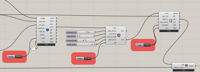
For people who are looking to make use of the powerful OpenStudio SDK to edit the details of their energy model, the learning curve just got significantly shallower. We have added a module that allows you to load and edit OSM models using the OpenStudio SDK right inside GHPython components, which enables you to bypass all of the Ruby environment setup and other challenges of setting up an OpenStudio Measure.
Click to read more
So, let’s say you wanted to tweak a property of your model that is not exposed in Honeybee. Like the setpoints in the air loop of the DOAS systems. Previously, you would have to do this by writing custom Ruby code that you’ve put inside of an OpenStudio Measure. Now, all that you need are a few lines of Python inside a GHPython component:
from ladybug_rhino.openstudio import load_osm, dump_osm

# load the Model from the OSM
model = load_osm(_osm)

# get all of the SetpointManagers and set their properties
setpt_managers = model.getSetpointManagerOutdoorAirResets()
for setpt in setpt_managers:
    setpt.setSetpointatOutdoorLowTemperature(_setp_at_low)
    setpt.setOutdoorLowTemperature(_low_temp)
    setpt.setSetpointatOutdoorHighTemperature(_setp_at_high)
    setpt.setOutdoorHighTemperature(_high_temp)

# save the edited OSM over the original one
osm = dump_osm(model, _osm)
… and all that you have to do is copy/paste this code into a GHPython component.
Dragonfly Features
Assign Ceiling Adjacencies and Separate Mid-Level Exposed Roofs
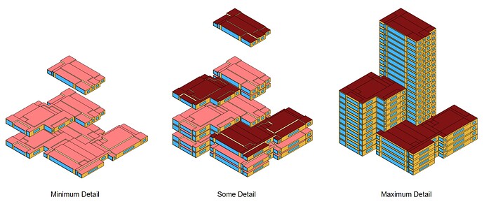
Many of us running large urban energy simulations with Dragonfly have been appreciative of the fact that whole building stories can be simulated with multipliers, cutting down the simulation time of urban districts to a small fraction of what they would be otherwise. However, there have also been requests at the other end of the spectrum, where people want to run production-level simulations that include the maximum detail. For those seeking the latter, you will be happy to know that two new features allow you to model even more detail.
Click to read more
The DF Separate Top Bottom component now has a separate_mid_ option, which can set exterior roof boundary conditions on middle floors that have no room above them. Furthermore, the DF Model To Honeybee component has a ciel_adj_ option to use surface boundary conditions between adjacent stories when not using multipliers.
Missing Legacy Features Targeted for the Next Stable Release
More Ladybug Visuals - We are still missing important ladybug visualizations such as radiation-related graphics, the wind profile, and analyses like shade benefit. We hope to get these in for the next release.
Dynamic Radiance Window Groups (3 and 5 Phase) - At the moment, there are components for dynamic Aperture and Shade groups but they are not used in any recipe. We hope to have 3-5-Phase and 5-Phase recipes implemented in the next release, which will be able to make use of these features to model dynamic shades.
Additional Energy Features - We are currently missing a few important energy simulation features like radiant HVAC, photovoltaics and more issues that can be seen on the honeybee-energy Github. We hope to work our way further down this list before the next release.
